MAE 318 - Homework 1
Problem 1: Modeling and simulating a mechanical system with translational motion [59 points]
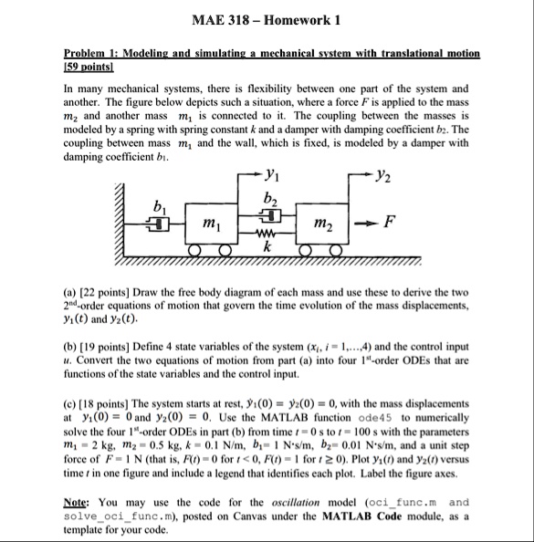
In many mechanical systems, there is flexibility between one part of the system and another. The figure below depicts such a situation, where a force F is applied to the mass m_(2) and another mass m_(1) is connected to it. The coupling between the masses is modeled by a spring with spring constant k and a damper with damping coefficient b_(2). The coupling between mass m_(1) and the wall, which is fixed, is modeled by a damper with damping coefficient b_(1).
(a) [22 points] Draw the free body diagram of each mass and use these to derive the two 2^(nd )-order equations of motion that govern the time evolution of the mass displacements, y_(1)(t) and y_(2)(t).
(b) [19 points] Define 4 state variables of the system ( x_(i),i=1,dots,4 ) and the control input u. Convert the two equations of motion from part (a) into four 1^(st )-order ODEs that are functions of the state variables and the control input.
(c) [18 points] The system starts at rest, y_(1)^(˙)(0)=y_(2)^(˙)(0)=0, with the mass displacements at y_(1)(0)=0 and y_(2)(0)=0. Use the MATLAB function ode 45 to numerically solve the four 1^(st )-order ODEs in part (b) from time t=0s to t=100s with the parameters m_(1)=2kg,m_(2)=0.5kg,k=0.1(N)/(m),b_(1)=1N*(s)/(m),b_(2)=0.01N*(s)/(m), and a unit step force of F=1N (that is, F(t)=0 for t<0,F(t)=1 for t>=0 ). Plot y_(1)(t) and y_(2)(t) versus time t in one figure and include a legend that identifies each plot. Label the figure axes.
Note: You may use the code for the oscillation model (oci_func.m and solve_oci_func.m), posted on Canvas under the MATLAB Code module, as a template for your code.