Bode plots
Given a system with transfer function H(s), Bode plots show the magnitude (|H(s)|) and phase (φ(H)(s) or φ(ω) responses of the system for s=jω, ω>0. H(ω) is found by setting s=jω in H(s). Transfer function H(s)=(an*s^n+an-1*s^(n-1)+...+a0)/(bm*s^m+bm-1*s^(m-1)+...+b0) in MATLAB is the command sys=tf(numerator, denominator),
where numerator=[[an,an-1,...,a0]] is the array of numerator coefficients and denominator=bmbm-1...b0 contains the denominator coefficients.
MATLAB Bode plot command variations:
bode(sys) plots |H(ω)| and φ(ω) vs frequency ω
bode(sys, w) plots |H(ω)| and φ(ω) vs the frequencies of the vector w.
[mag, phase, wout] = bode(sys, w) returns |H(ω)| in mag and φ(ω) in phase vs frequencies in w without plotting.
bode(sys1, ..., sysN, w) plots |H1(ω)|,...,HN(ω)|| and φ1(ω),...,φN(ω) vs frequencies specified by w on the same plots for ease of comparison.
w=logspace(a,b,N) sets loads w with N logarithmically-spaced frequencies between 10^a and 10^b; whereas, w=[w1,w2,...,wN] sets frequencies for the N specific frequencies provided.
For bode to provide a filter's magnitude and phase performance:
Convert the filter's H(ω) to the Laplace domain H(s) by setting jω to s.
Use tf command to input the transfer function H(s) in the variable sys.
Use bode(sys) to plot magnitude and phase responses, bode(sys, w) to plot magnitude and phase responses for frequencies in array w, or [mag, phase, wout] = bode(sys, w) to return the magnitude and phase of the response at each frequency in the vector w to variables mag and phase respectively, with wout containing the frequencies in w.
For the series RLC bandpass filter below,
the transfer function is H(ω)=(VR)/(VS)=(jRCω)/(-LCω^2+jRCω+1), or s-domain H(s)=(RC(s))/(LCs^2+RC(s)+1).
The resonant frequency ω0=(1)/(√(LC)), the quality factor Q=(ωL)/(R), and 3-dB bandwidth B=(R)/(L).
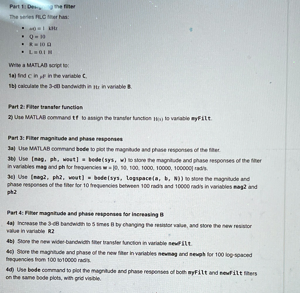
Part 1: Designing the filter
The series RLC filter has:
ω0=1kHz
Q=10
R=10Ω
L=0.1H
Write a MATLAB script to:
1a) find C in μF in the variable C,
1b) calculate the 3-dB bandwidth in Hz in variable B.
Part 2: Filter transfer function
Use MATLAB command tf to assign the transfer function H(s) to variable myFilt.
Part 3: Filter magnitude and phase responses
3a) Use MATLAB command bode to plot the magnitude and phase responses of the filter.
3b) Use [mag, ph, wout] = bode(sys, w) to store the magnitude and phase responses of the filter in variables mag and ph for frequencies w=[0,10,100,1000,10000,100000] rad/s.
3c) Use [mag2, ph2, wout] = bode(sys, logspace(a, b, N)) to store the magnitude and phase responses of the filter for 10 frequencies between 100 rad/s and 10000 rad/s in variables mag2 and ph2.
Part 4: Filter magnitude and phase responses for increasing
Part 1: Designing the filter
The series RLC filter has:
ω0=1kHz Q=10 R=10 L=0.1H
Write a MATLAB script to:
1a) find C in F in the variable C
1b) calculate the 3-dB bandwidth in Hz in variable B
Part 2: Filter transfer function
2) Use MATLAB command tf to assign the transfer function H(s) to variable myFilt
Part 3: Filter magnitude and phase responses 3a) Use MATLAB command bode to plot the magnitude and phase responses of the filter. 3b Use [mag, ph, wout]= bode(sys, w to store the magnitude and phase responses of the filter in variables mag and ph for frequencies w=[0,10,100,1000,10000,100000] rad/s 3c Use [mag2,ph2, wout]= bodesys,logspacea,b,Nto store the magnitude and phase responses of the filter for 10 frequencies between 100 rad/s and 10000 rad/s in variables mag2 and ph2
Part 4: Filter magnitude and phase responses for increasing B 4a) Increase the 3-dB bandwidth to 5 times B by changing the resistor value, and store the new resistor value in variable R2 4b) Store the new wider-bandwidth filter transfer function in variable newFilt 4c) Store the magnitude and phase of the new filter in variables newmag and newph for 100 log-spaced frequencies from 100 to 10000 rad/s 4d) Use bode command to plot the magnitude and phase responses of both myFilt and newFilt filters on the same bode plots, with grid visible.