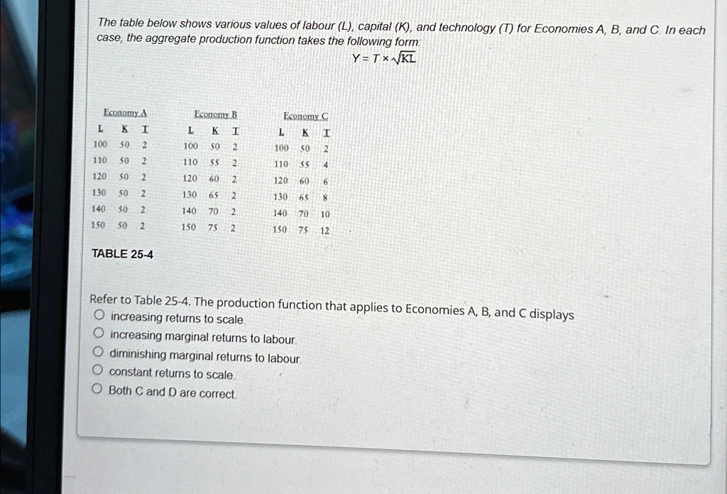
The table below shows various values of labor (L), capital (K), and technology (T) for Economies A, B, and C. In each case, the aggregate production function takes the following form: Y = T * √(K)L
[
�egin{array}{|c|c|c|c|c|c|c|c|c|}
hline
& ext{Economy A} & ext{Economy B} & ext{Economy C} \
hline
& L & K & T & L & K & T & L & K & T \
hline
& 100 & 50 & 2 & 100 & 50 & 2 & 100 & 50 & 2 \
& 110 & 50 & 2 & 110 & 55 & 2 & 110 & 55 & 4 \
& 120 & 50 & 2 & 120 & 60 & 2 & 120 & 60 & 6 \
& 130 & 50 & 2 & 130 & 65 & 2 & 130 & 65 & 8 \
& 140 & 50 & 2 & 140 & 70 & 2 & 140 & 70 & 10 \
& 150 & 50 & 2 & 150 & 75 & 2 & 150 & 75 & 12 \
hline
end{array}
]
TABLE 25-4
Refer to Table 25-4. The production function that applies to Economies A, B, and C displays increasing returns to scale, increasing marginal returns to labor, diminishing marginal returns to labor, constant returns to scale, or both C and D are correct.