Problem 2) 30 points-LQR Controller Development
For the simulation of Problem 1, linearize the system where CL is the input and h,
altitude, is the output/measurement. An example was shown in class on how to linearize
this model. Take those state-space matrices and develop a controller to reject
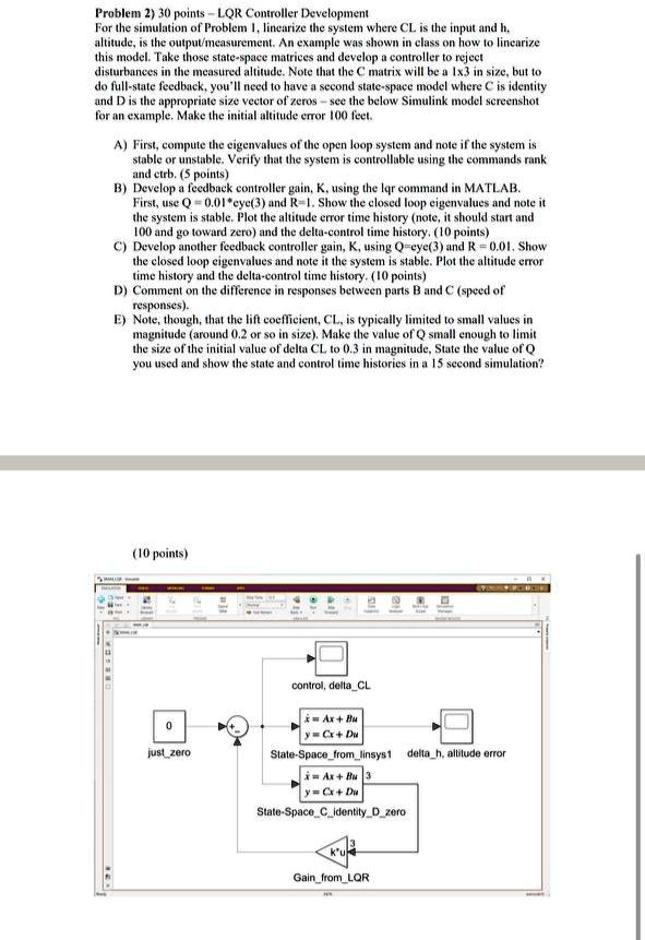
disturbances in the measured altitude. Note that the C matrix will be a 1x3 in size, but to
do full-state feedback, you'll need to have a second state-space model where C is identity
and D is the appropriate size vector of zeros - see the below Simulink model screenshot
for an example. Make the initial altitude error 100 feet.
A) First, compute the eigenvalues of the open loop system and note if the system is
stable or unstable. Verify that the system is controllable using the commands rank
and ctrb. (5 points)
B) Develop a feedback controller gain, K, using the lqr command in MATLAB.
First, use $Q = 0.01 \times eye(3)$ and $R = 1$. Show the closed loop eigenvalues and note it
the system is stable. Plot the altitude error time history (note, it should start and
100 and go toward zero) and the delta-control time history. (10 points)
C) Develop another feedback controller gain, K, using $Q = eye(3)$ and $R = 0.01$. Show
the closed loop eigenvalues and note it the system is stable. Plot the altitude error
time history and the delta-control time history. (10 points)
D) Comment on the difference in responses between parts B and C (speed of
responses).
E) Note, though, that the lift coefficient, CL, is typically limited to small values in
magnitude (around 0.2 or so in size). Make the value of Q small enough to limit
the size of the initial value of delta CL to 0.3 in magnitude, State the value of Q
you used and show the state and control time histories in a 15 second simulation?
(10 points)
0
just_zero
control, delta_CL
$x = Ax + Bu$
$y = Cx + Du$
State-Space_from_linsys1 delta_h, altitude error
$x = Ax + Bu$
$y = Cx + Du$
State-Space_C_identity_D_zero
k'u
3
Gain_from_LQR