Linear and Quadratic Trends in Time
Consider the deterministic time trend expressed as
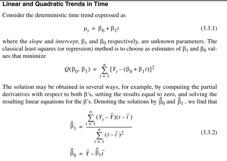
\(\mu_t = \beta_0 + \beta_1 t\)
(3.3.1)
where the slope and intercept, \(\beta_1\) and \(\beta_0\) respectively, are unknown parameters. The
classical least squares (or regression) method is to choose as estimates of \(\beta_1\) and \(\beta_0\) val-
ues that minimize
\(Q(\beta_0, \beta_1) = \sum_{t=1}^{n} [Y_t - (\beta_0 + \beta_1 t)]^2\)
The solution may be obtained in several ways, for example, by computing the partial
derivatives with respect to both \(\beta\)'s, setting the results equal to zero, and solving the
resulting linear equations for the \(\beta\)'s. Denoting the solutions by \(\hat{\beta}_0\) and \(\hat{\beta}_1\), we find that
\(\hat{\beta}_1 = \frac{\sum_{t=1}^{n} (Y_t - \bar{Y})(t - \bar{t})}{\sum_{t=1}^{n} (t - \bar{t})^2}\)
(3.3.2)
\(\hat{\beta}_0 = \bar{Y} - \hat{\beta}_1 \bar{t}\)