Problem 1
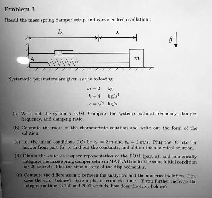
Recall the mass spring damper setup and consider free oscillation:
$l_0$
$x$
$g$
$A$
$m$
Systematic parameters are given as the following
$m = 2$ kg
$k = 4$ kg/s$^2$
$c = \sqrt{2}$ kg/s
(a) Write out the system's EOM. Compute the system's natural frequency, damped
frequency, and damping ratio.
(b) Compute the roots of the characteristic equation and write out the form of the
solution.
(c) Let the initial conditions (IC) be $x_0 = 2$ m and $v_0 = 2$ m/s. Plug the IC into the
answer from part (b) to find out the constants, and obtain the analytical solution.
(d) Obtain the state state-space representation of the EOM (part a), and numerically
integrate the mass spring damper setup in MATLAB under the same initial condition
for 20 seconds. Plot the time history of the displacement $x$.
(e) Compute the difference in $x$ between the analytical and the numerical solution. How
does the error behave? Save a plot of error vs. time. If you further increase the
integration time to 200 and 2000 seconds, how does the error behave?