Ex 5.5: Function optimization. Consider the function f(x,y)=x^(2)+20y^(2) shown in Fig-
ure 5.63a. Begin by solving for the following:
Calculate gradf, i.e., the gradient of f.
Evaluate the gradient at x=-20,y=5.
Implement some of the common gradient descent optimizers, which should take you from
the starting point x=-20,y=5 to near the minimum at x=0,y=0. Try each of the
following optimizers:
Standard gradient descent.
Gradient descent with momentum, starting with the momentum term as
ho =0.99.
Adam, starting with decay rates of �eta _(1)=0.9 and b_(2)=0.999.
Play around with the learning rate alpha . For each experiment, plot how x and y change over
time, as shown in Figure 5.63b.
How do the optimizers behave differently? Is there a single learning rate that makes all
the optimizers converge towards x=0,y=0 in under 200 steps? Does each optimizer
monotonically trend towards x=0,y=0 ?Figure 5.63 Function optimization: (a) the contour plot of f(x,y)=x^(2)+20y^(2) with
the function being minimized at (0,0);(b) ideal gradient descent optimization that quickly
converges towards the minimum at x=0,y=0.
Would batch normalization help in this case?
Note: the following exercises were suggested by Matt Deitke.
Ex 5.5: Function optimization. Consider the function f(x,y)=x^(2)+20y^(2) shown in Fig-
ure 5.63a. Begin by solving for the following:
Calculate gradf, i.e., the gradient of f.
Evaluate the gradient at x=-20,y=5.
Implement some of the common gradient descent optimizers, which should take you from
the starting point x=-20,y=5 to near the minimum at x=0,y=0. Try each of the
following optimizers:
Standard gradient descent.
Gradient descent with momentum, starting with the momentum term as
ho =0.99.
Adam, starting with decay rates of �eta _(1)=0.9 and b_(2)=0.999.
Play around with the learning rate alpha . For each experiment, plot how x and y change over
time, as shown in Figure 5.63b.
How do the optimizers behave differently? Is there a single learning rate that makes all
the optimizers converge towards x=0,y=0 in under 200 steps? Does each optimizer
monotonically trend towards x=0,y=0 ?
Start Her
-20
-10
0
10
20
Time
(a)
(b)
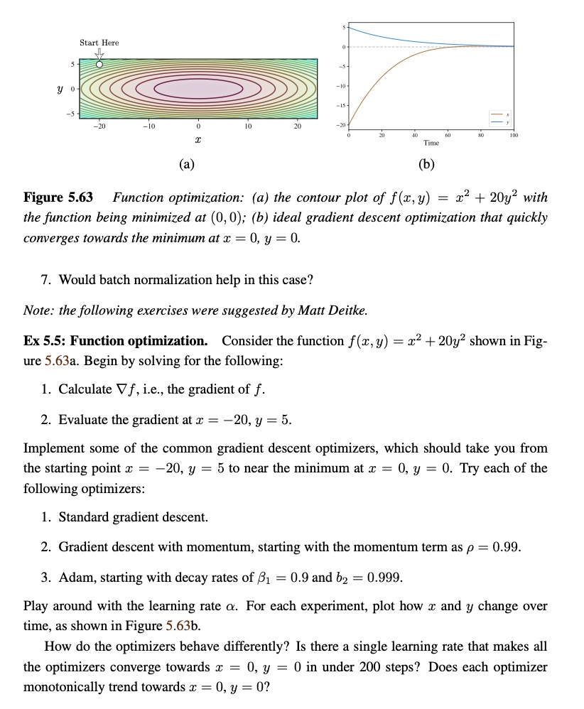
Figure 5.63 Function optimization: (a) the contour plot of f(x,y) = x2 + 20y2 with the function being minimized at (0, 0); (b) ideal gradient descent optimization that quickly converges towards the minimum at x = 0, y = 0.
7. Would batch normalization help in this case?
Note: the following exercises were suggested by Matt Deitke.
Ex 5.5: Function optimization. Consider the function f(x, y) = x2 + 20y2 shown in Fig. ure 5.63a. Begin by solving for the following:
1. Calculate V f, i.e., the gradient of f.
2. Evaluate the gradient at x = --20, y = 5.
Implement some of the common gradient descent optimizers, which should take you from the starting point x = -20, y = 5 to near the minimum at = 0, y = 0. Try each of the following optimizers:
1. Standard gradient descent.
2. Gradient descent with momentum, starting with the momentum term as p = 0.99
3. Adam, starting with decay rates of =0.9 and b2=0.999
Play around with the learning rate a. For each experiment, plot how x and y change over time, as shown in Figure 5.63b.
How do the optimizers behave differently? Is there a single learning rate that makes all
the optimizers converge towards x = 0, y = 0 in under 200 steps? Does each optimizer
monotonically trend towards x = 0, y = 0?