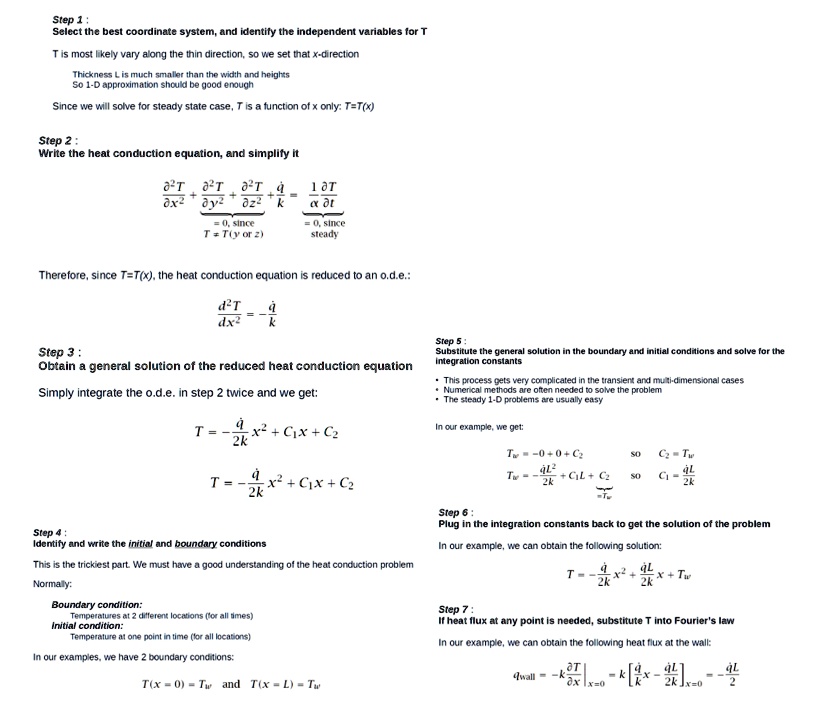
please use phyton program. Use numerical methods to find the temperature distribution inside
the concrete slab in the following simple 1D heat transfer problem
and compare with the analytical solution. Analytical solution steps are below.
A large, thin concrete slab of thickness L is "setting." Setting is an
exothermic process that releases heat volumetrically, q^(˙)((W)/(m^(3))). The
outside surfaces are kept at the ambient temperature, so T_(w)=T_(infty ).Since we will solve for steady state case, T is a function of x only: T=T(x)
Step 2 :
Write the heat conduction equation, and simplify it
(del^(2)T)/(delx^(2))+ubrace((del^(2)T)/(dely^(2))+(del^(2)T)/(delz^(2))ubrace)_({(:[=0, since ]),(T=T(y or z)):})+((q^(˙)))/(k)=ubrace((1)/(alpha )(delT)/(delt)ubrace)_({(:[=0, since ]),( steady ):})
Therefore, since T=T(x), the heat conduction equation is reduced to an o.d.e.:
(d^(2)T)/(dx^(2))=-((q^(˙)))/(k)
Step 3 :
Obtain a general solution of the reduced heat conduction equation
Simply integrate the o.d.e. in step 2 twice and we get:
T=-((q^(˙)))/(2k)x^(2)+C_(1)x+C_(2)
T=-((q^(˙)))/(2k)x^(2)+C_(1)x+C_(2)
Step 4 :
Identify and write the initial and boundary conditions
This is the trickiest part. We must have a good understanding of the heat conduction problem
Normally:
Boundary condition:
Temperatures at 2 different locations (for all imes)
Initial condition:
Temperature at one point in time (for all locations)
In our examples, we have 2 boundary conditions:
T(x=0)=T_(w), and ,T(x=L)=T_(w)
Step 5 :
Substitute the general solution in the boundary and initial conditions and solve for the
integration constants
This process gets very complicated in the transient and muti-dimensional cases
Numerical methods are often needed to solve the problem
The steady 1-D problems are usually easy
In our example, we get:
T_(w)=-0+0+C_(2) so C_(2)=T_(w)
T_(w)=-((q^(˙))L^(2))/(2k)+C_(1)L+ubrace(C_(2)ubrace)_()=T_(w) so C_(1)=((q^(˙))L)/(2k)
Step 6 :
Plug in the integration constants back to get the solution of the problem
In our example, we can obtain the following solution:
T=-((q^(˙)))/(2k)x^(2)+((q^(˙))L)/(2k)x+T_(w)
Step 7 :
If heat flux at any point is needed, substitute T into Fourier's law
In our example, we can obtain the following heat flux at the wall:
q_(wall )=-k(delT)/(delx)|_(x)=0=k[((q^(˙)))/(k)x-((q^(˙))L)/(2k)]_(x)=0=-((q^(˙))L)/(2)pppppp
Step 1 : Select the best coordinate system, and identify the independent variables for T
T is most likely vary along the thin direction, so we set that -direction
Thickness L is much smaller than the width and heights So 1-D approximation should be good enough
Since we will solve for steady state case, T is a function of x only: T=T()
Step 2 : Write the heat conduction e quation, and simplify it
TTT .9 ax2 Dy2*dz2 =0,since T T(y or z)
1T 1 = 0, since steady
Therefore,since T=T(x), the heat conduction equation is reduced to an o.d.e.:
dx-2
Step 5 : Substitute the general solution in the boundary and initial conditions and solve for the integration constants
Step 3 : Obtain a general solution of the reduced heat conduction equation
This process gets very complicated in the transient and multi-dimensional cases Numerical methods are often needed to solve the problem The steady 1-D problems are usually easy
Simply integrate the o.d.e. in step 2 twice and we get:
a T = 2 + Cx + C2 2k
In our example, we get:
T= =0 +0+C2 qL2 Ta = + CL + C2
so
C2 = T qL
a 2 + Cx + C2 2k
so
T=
Step 6:
Step 4: Identify and write the initial and boundary conditions
In our example, we can obtain the following solution:
This is the trickiest part. We must have a good understanding of the heat conduction problem
T = 2k *
+ Ta 2k
Normally:
Boundary condition: Temperatures at 2 different locations (for all times) Initial condition: Temperature at one point in time (for all locations)
Step 7 : If heat flux at any point is needed, substitute T into Fourier's law
In our example,we can obtain the following heat flux at the wall:
In our examples, we have 2 boundary conditions:
T(x = 0) = TandT(x = L) =T