Ace - AI Tutor
Ask Our Educators
Textbooks
My Library
Flashcards
Scribe - AI Notes
Notes & Exams
Download App
diego green

diego g.

Divider

Questions asked

BEST MATCH

free cash flow is defined as? a cash flows available for payments to stockholders of a firm after the firm has made payments ot all others with claims against it

View Answer
divider
BEST MATCH

Two current-carrying wires are separated by a distance 0.50 m. Wire 1 has a current of 1.5 A and wire 2 has a current of 2.5 A but flowing in the opposite direction

View Answer
divider
BEST MATCH

don't use third party content 80. How is cut-off frequency determined in AC measurement instruments?

View Answer
divider
BEST MATCH

Find the domain of the logarithmic function and then graph the function. y = \ln (5x+8) Find the domain of the function. (Type your answer in interval notation. Use integers or fractions for any numbers in the expression. Simplify your answer.)

View Answer
divider
BEST MATCH

Assuming an upward-sloping, short-run aggregate supply curve, a decrease in government spending results in _ in equilibrium output and _ in equilbrium prices in the short run

View Answer
divider
BEST MATCH

The circuit in the figure below has been connected for a long time. Let $R_1 = 8.80 \Omega$ and $R_2 = 5.40 \Omega$. 1.00 $\Omega$ $R_1$ + 1.00 $\mu F$ 10.0 V $R_2$ 2.00 $\Omega$ (a) What is the potential difference across the capacitor? 6.586 V (b).If.the battery is disconnected from the circuit, over what time interval does the capacitor discharge to one-half its initial voltage? X Enter a number. differs from the correct answer by more than 100%. $\mu s$

View Answer
divider
BEST MATCH

2. [8 pts] Find R<sub>T</sub> = _____ Show at least 3 intermediate steps (circuit diagrams) showing the series-parallel reductions 40. Calculate the total resistance in the circuit shown in Figure 6.58. \Omega FIGURE 6.58 R<sub>7</sub> 8.2 k\Omega R<sub>5</sub> 10 k\Omega W R<sub>6</sub> 3.3 k\Omega W R<sub>8</sub> 11 k\Omega R<sub>4</sub> 10 k\Omega R<sub>1</sub> 22 k\Omega R<sub>2</sub> 11 k\Omega R<sub>9</sub> 8.8 k\Omega R<sub>3</sub> 4.7 k\Omega

View Answer
divider
BEST MATCH

Density (kg/m³) Water = 1,000 Corn syrup = 1,408 3 mm glass bead = 2,430 Viscosity (kg/s\cdot m) Water = 0.890 \times 10^{-3} Corn syrup = 7

View Answer
divider
BEST MATCH

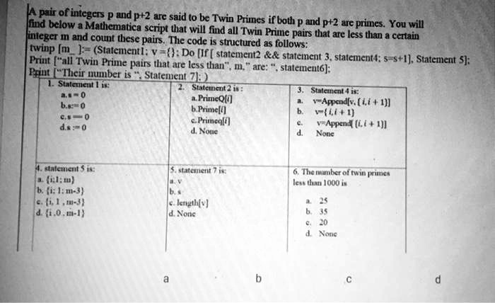
A pair of integers p and p+2 are said to be Twin Primes if both p and p+2 are primes. You will find below a Mathematica script that will find all Twin Prime pairs that are less than a certain integer m and count these pairs. The code is structured as follows: twinp [m]:= (Statement1: v={}; Do [If [statement2 && statement 3, statement4; s=s+1], Statement 5]; Print ["all Twin Prime pairs that are less than", m, " are: ", statement6]; Print ["Their number is", Statement 7]:) 1. Statement 1 is: a.s=0 b.s<0 c.s=0 d.s:=0 2. Statement 2 is: a. PrimeQ[i] b.Prime[i] c.Primeq[i] d. None 3. Statement 4 is: a. v=Append[v, {i, i+1}] b. v={i,i+1} c. v=Append[{i, i+1}] d. None 4. statement 5 is: a. {i,1:m} b. {i,1:m-3} c. {i, 1, m-3} d. {i,0,m-1} 5. statement 7 is: a. v b. s c. length[v] d. None 6. The number of twin primes less than 1000 is a. 25 b. 35 c. 20 d. None a b c d
View Answer
divider
BEST MATCH

The following model investigates the relationship between annual wage in logarithm form (LWAGE) and years of work experience (EXPER), years of schooling (EDUC), whether an individual is a union member (UNION) using data for 1,260 individuals. UNION is a dummy variable, with 0 meaning that the individual is not a union member and 1 denoting otherwise. Table Six provides the results from a simple linear regression model, while Tables Seven and Eight present results from diagnostic testing of this model. Table Nine presents further analysis. Table Six Dependent Variable: LWAGE Method: Least Squares Sample: 1,260 Included observations: 1,260 Variable Std. Error t-Statistic Prob. 0.277500 0.081437 3.407558 0.0007 EXPER 0.017670 0.001253 14.10546 0.0000 EDUC 0.079169 0.005714 13.85586 0.0000 UNION 0.238594 0.033222 7.181775 0.0000 Table Seven Heteroskedasticity Test: Breusch-Pagan-Godfrey Null hypothesis: Homoskedasticity F-statistic: 4.279287 Prob. F(3,1256): 0.0051 Obs*R-squared: 0.0052 Prob. Chi-Square(3): 0.0001 Scaled explained SS: 20.38491 Prob. Chi-Square(3): 0.0002 Table Eight Heteroskedasticity Test: White Null hypothesis: Homoskedasticity F-statistic: 2.404967 Prob. F(8,1251): 0.0141 Obs*R-squared: 19.08464 Prob. Chi-Square(8): 0.0144 Scaled explained SS: 30.51657 Prob. Chi-Square(8): 0.0002 Further analysis generated the findings reported in Table Nine. Table Nine Dependent Variable: LWAGE Method: Least Squares Sample: 1,260 Included observations: 1,260 Huber-White-Hinkley (HC1) het errors and covariance Variable C EXPER EDUC UNION Coefficient Std. Error t-Statistic Prob. 0.277500 0.083471 3.324504 0.0009 0.017670 0.001251 14.12661 0.0000 0.079169 0.005872 13.48330 0.0000 0.238594 0.030783 7.750763 0.0000 (e) Explain what is meant by heteroskedasticity and discuss why this problem needs to be addressed if detected in a model. (b) Explain in detail the approach of Weighted Least Squares used by applied economists to address heteroskedasticity in empirical work. (c) Provide a detailed and comparative account of the two tests of heteroskedasticity (the Breusch-Pagan test and the White test). According to the outputs presented above in Tables Seven and Eight, what are your conclusions on the two heteroskedasticity detecting tests? By comparing Tables Six and Nine, discuss the impacts on the estimation results if heteroskedasticity is present.

View Answer
divider