I know Chegg guidelines say only one answer, but I've posted the first question nearly 5 times and no one has bothered to help me. If anyone can help me with a few of these questions, I'd really appreciate it. Need help with Q1d the most :)
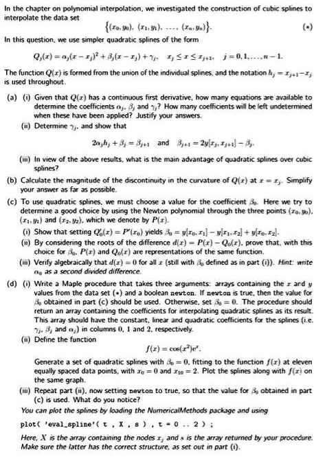
In the chapter on polynomial interpolation, we investigated the construction of cubic splines to interpolate the data set {xw, x1, yx, x3, n}. In this question, we use simpler quadratic splines of the form:
Q(x) = ax^2 - bx + cx + d, j = 0, 1, ..., n-1.
The function Q is formed from the union of the individual splines, and the notation h = x_i+1 - x_i is used throughout. Given that Q has a continuous first derivative, how many equations are available to determine the coefficients? And how many coefficients will be left undetermined when these have been applied? Justify your answers. Determine j and show that:
2h + 3 = x_i+1 - x_i and 3h + 1 = 2yx_i+1 - yx_i.
In view of the above results, what is the main advantage of quadratic splines over cubic splines? Calculate the magnitude of the discontinuity in the curvature of Q(x) at x = S. Simplify your answer as far as possible.
To use quadratic splines, we must choose a value for the coefficient a. Here we try to determine a good choice by using the Newton polynomial through the three points (x0, y0), (x1, y1), and (x2, y2), which we denote by P(x). Show that setting Q(x) = P(x) yields y[x0] = y[x1] = y[x2].
By considering the roots of the difference d(z) = P(z) - Q(z), prove that with this choice for P(x) and Q(x), they are representations of the same function.
Write a Maple procedure that takes three arguments: arrays containing the x and y values from the data set, and a boolean newton. If newton is true, then the value for a obtained in part c should be used. Otherwise, set a = 0. The procedure should return an array containing the coefficients for interpolating quadratic splines as its result. This array should have the constant, linear, and quadratic coefficients for the splines, i.e., a, b, and c in columns 0, 1, and 2, respectively.
Define the function f(x) = cos(x). Generate a set of quadratic splines with h = 0.2, fitting to the function f(x) at eleven equally spaced data points, with x0 = 0 and x1 = 2. Plot the splines along with f(x) on the same graph.
What do you notice? You can plot the splines by loading the NumericalMethods package and using ploteval_spline(t, X, s), where X is the array containing the nodes and s is the array returned by your procedure. Make sure the latter has the correct structure, as set out in part o.