Ace - AI Tutor
Ask Our Educators
Textbooks
My Library
Flashcards
Scribe - AI Notes
Notes & Exams
Download App
name8904 07

name8904 0.

Divider

Questions asked

ANSWERED

Nick Johnson verified

Numerade educator

d. Sum of products 4. The __________ line for a set of data is the line that comes the closest to the most data points in a scatterplot of the data. a. Slope b. Curve c. Best-fit d. Intercept 5. We cannot draw direct/causal conclusions in __________ studies as well as we can in experiments. a. Case b. Quasi-experimental c. Ethnographic d. Correlational 6. A __________ of 0 indicates no relationship between variables. a. Tukey ad hoc b. Kendall's Tau-B c. Somer's d d. Pearson r 7. Which correlation is stronger?

View Answer
divider
ANSWERED

Nick Johnson verified

Numerade educator

1. The larger the numerical value of Pearson's r, the __________ the relationship. a. Stronger b. Weaker c. More Positive d. More Negative 2. We cannot determine this from correlation and regression tests. a. Causation b. Standard effect size c. Sum of Squares d. Product effect size 3. The __________ is a measure of how much of the variability in one measure is explained by the value of the other measure. a. R² b. Pearson's r c. Correlation d. Sum of products

View Answer
divider
INSTANT ANSWER

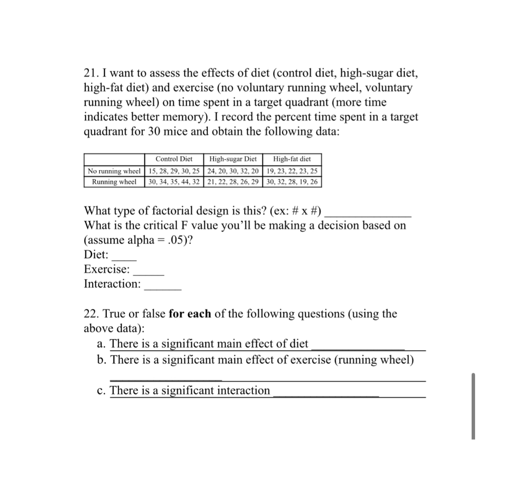
21. I want to assess the effects of diet (control diet, high-sugar diet, high-fat diet) and exercise (no voluntary running wheel, voluntary running wheel) on time spent in a target quadrant (more time indicates better memory). I record the percent time spent in a target quadrant for 30 mice and obtain the following data: \begin{tabular}{|c|c|c|c|} \hline & Control Diet & High-sugar Diet & High-fat diet \\ \hline No running wheel & \( 15,28,29,30,25 \) & \( 24,20,30,32,20 \) & \( 19,23,22,23,25 \) \\ \hline Running wheel & \( 30,34,35,44,32 \) & \( 21,22,28,26,29 \) & \( 30,32,28,19,26 \) \\ \hline \end{tabular} What type of factorial design is this? (ex: \# \( \mathrm{x} \) \#) \( \qquad \) What is the critical \( \mathrm{F} \) value you'll be making a decision based on (assume alpha \( =.05 \) )? Diet: \( \qquad \) Exercise: \( \qquad \) Interaction: \( \qquad \) 22. True or false for each of the following questions (using the above data): a. There is a significant main effect of diet b. There is a significant main effect of exercise (running wheel) c. There is a significant interaction
View Answer
divider
INSTANT ANSWER

19. Given the following data, test (at an alpha of 0.05 ) whether type of music affects heart rate (measured in beats per minute, bpm). \begin{tabular}{|c|c|c|c|c|} \hline Participant & Rock & Classical & Heavy Metal & ROW MEANS = \\ \hline\( / \) & 70 & 64 & 90 & 74.67 \\ \hline 2 & 78 & 69 & 85 & 77.33 \\ \hline 3 & 80 & 72 & 67 & 73 \\ \hline 4 & 82 & 65 & 100 & \( \mathbf{8 2 . 3 3} \) \\ \hline 5 & 81 & 67 & 120 & \( \mathbf{8 9 . 3 3} \) \\ \hline 6 & 80 & 58 & 98 & 78.67 \\ \hline GROUP MEANS = & \( \mathbf{7 8 . 5} \) & \( \mathbf{6 5 . 8 3} \) & \( \mathbf{9 3 . 3 3} \) & \\ \hline & & & & \\ \hline \end{tabular} Grand/Total mean \( =79.22 \) a. What is the null hypothesis? a. \( \mu 1=\mu 2=\mu 3 \) b. At least one mean differs b. What is the alternative hypothesis? a. \( \mu 1=\mu 2=\mu 3 \) b. At least one mean differs c. What is the critical value (from \( \mathrm{F} \) table): d. Fill in the ANOVA summary Table: \begin{tabular}{|c|c|c|c|c|} \hline SOURCE & \begin{tabular}{c} SUMS OF \\ SQUARES \end{tabular} & DF & MS (VARIANCE) & F \\ \hline \begin{tabular}{c} Between groups \\ (bye of music) \end{tabular} & - & 2 & 1136.72 & - \\ \hline Error & 1235.89 & - & 123.59 & \\ \hline Total & 4035.11 & 17 & & \\ \hline \end{tabular} e. What is our final decision? a. We reject the null hypothesis. There is sufficient evidence to conclude that type of music has a significant effect on heart rate, \( \mathrm{p}< \) 0.05 . b. We fail to reject the null hypothesis. There is insufficient evidence to conclude that type of music has an effect on heart rate, \( p \) \( >0.05 \). f. Run a post hoc test on this data (using a Tukey correction) and tell me which music pair has the lowest p value. 20. How many groups/cells are in a \( 4 \times 2 \) Factorial ANOVA design?

View Answer
divider
ANSWERED

Caroline Mcclure verified

Numerade educator

16. Which measure of central tendency is easily influenced by outliers? 17. Using the following data, | 5 | 2 | 4 | 7 | 3 | 9 | 5 | 5 | 11 | 9 | Calculate the: a. Mean: __________ b. Median: __________ c. Mode: __________ d. Variance: __________ e. Standard Deviation: __________ f. Range: __________ 18. Complete the following one-way, between-subjects ANOVA summary table: | SOURCE | SUMS OF SQUARES | DF | MS (VARIANCE) | F | | :--- | :---: | :---: | :---: | :---: | | Between-groups | 60 | | 15 | 16 | | Error | | 16 | | | | Total | 75 | 20 | | |

View Answer
divider
INSTANT ANSWER

15. I'm interested in seeing whether or not online supplementary material helps students achieve higher grades in statistics. I assign 10 students into a class using an online textbook resource whereas 10 separate students are assigned into a class using just the textbook. I recorded their final course average (final course grade). Using the following data (testing at an alpha of . 05 ), assess whether those that used the online resources + textbook (group 1) did better than those just using the textbook (group 2 ). \begin{tabular}{|c|c|} \hline Online resources + Textbook (group 1) & Just textbook (group 2) \\ \hline 95 & 90 \\ \hline 90 & 86 \\ \hline 92 & 75 \\ \hline 92 & 87 \\ \hline 84 & 85 \\ \hline 86 & 83 \\ \hline 91 & 90 \\ \hline 92 & 83 \\ \hline 80 & 85 \\ \hline 82 & 78 \\ \hline \end{tabular} a. Independent variable: \( \qquad \) b. Dependent variable: \( \qquad \) c. What is the null hypothesis? a. \( \mu 1=\mu 2 \) b. \( \mu 1 \neq \mu 2 \) c. \( \mu 1>\mu 2 \) d. \( \mu 1<\mu 2 \) d. What is the alternative hypothesis? a. \( \mu 1=\mu 2 \) b. \( \mu 1 \neq \mu 2 \) c. \( \mu 1>\mu 2 \) d. \( \mu 1<\mu 2 \) e. Degrees of freedom: \( \qquad \) f. Critical value (from the \( t \) table): \( \qquad \) g. Obtained test statistic: \( \qquad \) h. Using Jamovi, what is the p value associated with our test statistic? \( \qquad \) i. What can we conclude? a. We reject the null hypothesis. There is sufficient evidence to conclude that type of resource has a significant effect on final exam grades, \( \mathrm{p}<0.05 \). b. We fail to reject the null hypothesis. There is insufficient evidence to conclude that type of resource has an effect on final exam grades, \( \mathrm{p}>0.05 \)

View Answer
divider
INSTANT ANSWER

13. I am studying whether or not the type of container you're drinking from affects how much water you drink. I divide 30 students into two groups: one group drinks water from a bottle, and the other drinks water from a one-gallon jug. I measure the amount of time it takes (in seconds) for the groups to drink \( 500 \mathrm{~mL} \) of water. a. What is the independent variable? a. Type of container b. Time it takes to consume the water b. What is the dependent variable? a. Type of container b. Time it takes to consume the water 14. The average national salary is 45,000 (in this example, 45 represents 45,000). I take a sample of 14 individuals in San Antonio and measure their average salary and obtain the following data: \begin{tabular}{|c|c|c|c|c|c|c|c|c|c|c|c|c|c|c|} \hline \begin{tabular}{c} Individu \\ al \end{tabular} & 1 & 2 & 3 & 4 & 5 & 6 & 7 & 8 & 9 & 10 & 11 & 12 & 13 & 14 \\ \hline Salary & 45 & 56 & 60 & 65 & 60 & 63 & 54 & 51 & 27 & 29 & 34 & 35 & 35 & 37 \\ \hline \end{tabular} I conducted a test (at an alpha of .05) to answer whether or not those in San Antonio's salary is significantly greater than the national average. One Sample T-Test \begin{tabular}{lcccc} \multicolumn{2}{l}{ One Sample T-Test } \\ & & & \\ \hline & Statistic & df & P \\ \hline Salary & Student's & 0.42 & 13.00 & 0.341 \\ \hline \end{tabular} Note. \( H_{2} \mu>45 \) a. Based on the output above, what can I conclude? a. We reject the null hypothesis. There is sufficient evidence to conclude that our sample is significantly different from the national average, \( \mathrm{p}<0.05 \). b. We fail to reject the null hypothesis. There is insufficient evidence to conclude that our sample is different from the national average, \( p>0.05 \).

View Answer
divider
INSTANT ANSWER

10. A company sells bags of candy with five different flavors: apple, lime, cherry, orange, and grape. Each bag contains 200 pieces of candy. We want to test whether or not there is a significant difference (at an alpha of 0.01 ) between the actual, observed amounts of each flavor and what we would expect if each candy flavor was equally represented. We count the number of flavored candies and get the following counts: \begin{tabular}{|c|c|c|c|c|} \hline Apple & Lime & Cherry & Orange & Grape \\ \hline 32 & 25 & 53 & 40 & 50 \\ \hline \end{tabular} a. What are our degrees of freedom for this example? b. What is our critical (from the chi-square table) value? c. What is our obtained chi-square value? d. What can we conclude? a. We reject the null hypothesis. There is sufficient evidence to conclude that there is a preference for at least one of the flavors. b. We fail to reject the null hypothesis. There is insufficient evidence to conclude that there is a preference between flavors. 11. If you go to a doctor's office and they measure your height, this variable is measured on what type of scale? a. Nominal b. Ordinal c. Interval d. Ratio 12. If you go to a doctor's office and they ask you if you smoke (Yes/No), this variable is measured on what type of scale? a. Nominal b. Ordinal c. Interval d. Ratio

View Answer
divider
INSTANT ANSWER

8. I'm interested in assessing whether someone's resting heart rate \( (\mathrm{X}) \) is related to how fast they are able to finish running a \( 5 \mathrm{k} \) race ( \( 5 \mathrm{k} \) is 3.1 miles) (Y). I gather data from a set of runners and want to see whether, at an alpha of 0.05 , there is a significant relationship between resting heart rate and finish time. Use the data below to answer this question: \begin{tabular}{|c|c|} \hline Resting Heart Rate (measured in beats/min) (X) & Finish Time (measured in minutes) (Y) \\ \hline 54 & 30 \\ \hline 65 & 33 \\ \hline 60 & 35 \\ \hline 60 & 32 \\ \hline 75 & 35 \\ \hline 70 & 36 \\ \hline 80 & 45 \\ \hline 60 & 36 \\ \hline 55 & 29 \\ \hline 55 & 27 \\ \hline 60 & 30 \\ \hline \end{tabular} a. What is the null hypothesis? a. \( \rho=0 \) b. \( \rho \neq 0 \) c. \( \rho>0 \) d. \( \rho<0 \) b. What is the alternative hypothesis? a. \( \rho=0 \) b. \( \rho \neq 0 \) c. \( \rho>0 \) d. \( \rho<0 \) c. What are the degrees of freedom for this problem? What is the critical \( \mathrm{R} \) value? \( \qquad \) \( \qquad \) d. What is the Pearson correlation coefficient? Is it strong or weak? Positive or negative? \( \qquad \) \( \qquad \) e. What can we conclude? a. Reject the null hypothesis. There is sufficient evidence to indicate there is a significant relationship between resting heart rate and finish time. b. Fail to reject the null hypothesis. There is insufficient evidence to indicate there is a significant relationship between resting heart rate and finish time. f. What is the \( R^{2} \) value (give this value as a decimal)? What does it represent in this problem's context? (Interpret it)

View Answer
divider
ANSWERED

Benjamin Densmore verified

Numerade educator

d. Pearson r 7. Which correlation is stronger? a. r = -0.8 or r = 0.8 b. r = -0.5 or r = 0.4 c. r = 1 or r = -1.5

View Answer
divider