Texts:
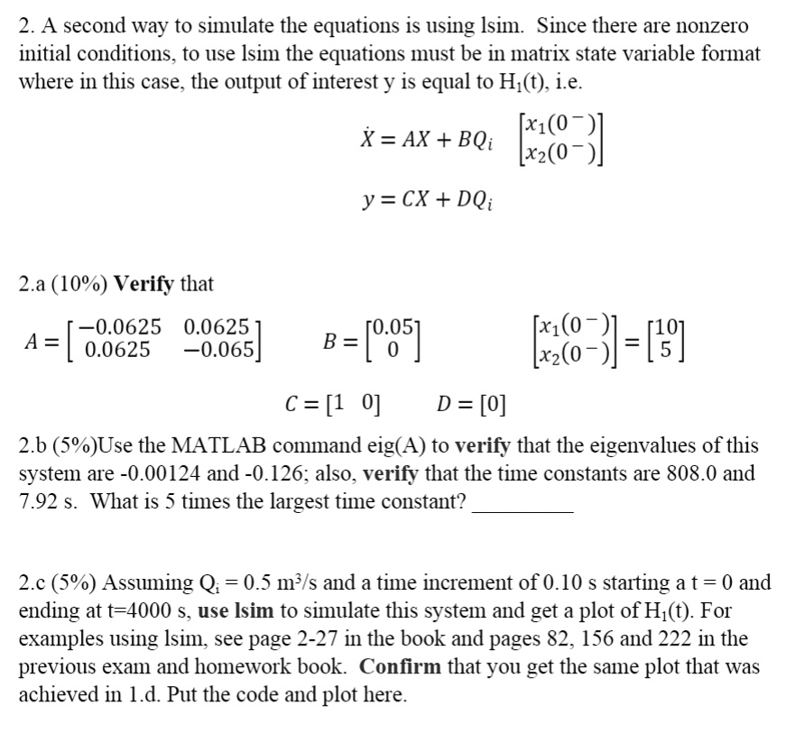
2. A second way to simulate the equations is using lsim. Since there are nonzero initial conditions, to use lsim, the equations must be in matrix state variable format where in this case, the output of interest y is equal to Hi(t), i.e.
[x(0)] X = AX + BQi x2(0)
y = CX + DQi
2.a (10%) Verify that
[-0.0625 0.0625] [0.05] A B = [(8-3) -1] [0.0625 -0.065 0] C = [1 0] D = [0]
2.b (5%) Use the MATLAB command eig(A) to verify that the eigenvalues of this system are -0.00124 and -0.126; also, verify that the time constants are 808.0 and 7.92 s. What is 5 times the largest time constant?
2.c (5%) Assuming Qi = 0.5 m3/s and a time increment of 0.10 s starting at t = 0 and ending at t = 4000 s, use lsim to simulate this system and get a plot of H(t). For examples using lsim, see page 2-27 in the book and pages 82, 156, and 222 in the previous exam and homework book. Confirm that you get the same plot that was achieved in 1.d. Put the code and plot here.