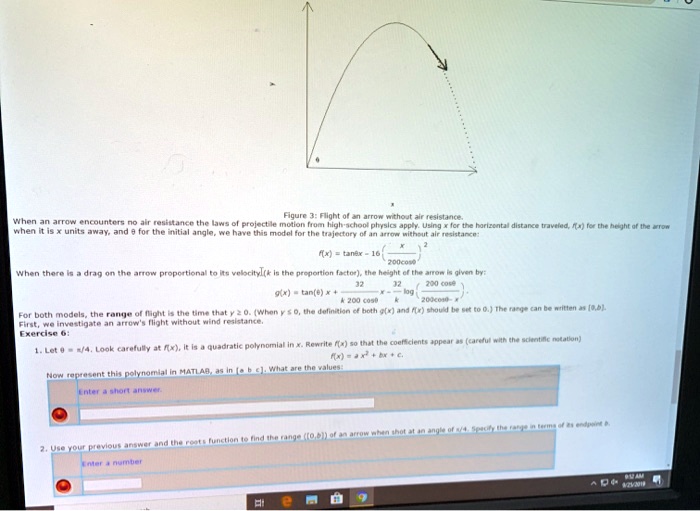
Figure 3: Flight of an arrow without air resistance.
When an arrow encounters no air resistance the laws of projectile motion from high-school physics apply. Using x for the horizontal distance traveled, f(x) for the height of the arrow
when it is x units away, and \theta for the initial angle, we have this model for the trajectory of an arrow without air resistance:
\begin{equation}
f(x) = \tan\theta x - \frac{16}{200\cos\theta}x^2
\end{equation}
When there is a drag on the arrow proportional to its velocity(k is the proportion factor), the height of the arrow is given by:
\begin{equation}
g(x) = \tan(\theta) x + \frac{200\cos\theta}{32} - \frac{32}{k} \log\left(\frac{200\cos\theta}{200\cos\theta - kx}\right)
\end{equation}
For both models, the range of flight is the time that y \ge 0. (When y \le 0, the definition of both g(x) and f(x) should be set to 0.) The range can be written as [0,b].
First, we investigate an arrow's flight without wind resistance.
Exercise 6:
1. Let \theta = \frac{\pi}{4}. Look carefully at f(x), it is a quadratic polynomial in x. Rewrite f(x) so that the coefficients appear as (careful with the scientific notation)
$f(x) = ax^2 + bx + c$
Now represent this polynomial in MATLAB, as in [a b c]. What are the values:
Enter a short answer.
2. Use your previous answer and the roots function to find the range ([0,b]) of an arrow when shot at an angle of \frac{\pi}{4}. Specify the range in terms of its endpoint b
Enter a number