I want to summarize the article and also solve the existing equations using MATLAB and also explain and interpret the results in the table and how to access them. Is it possible to improve this model?
8--8
+;+ x-,
0.16) o.m
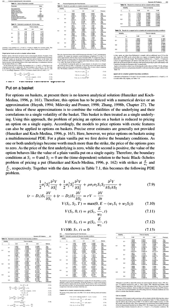
Put on a basket For options on baskets, at present there is no known analytical solution (Hunziker and Koch- Medina, 1996, p. 161). Therefore, this option has to be priced with a numerical device or an approximation (Huynh, 1994; Milevsky and Posner, 1998; Zhang, 1998b, Chapter 27). The basic idea of these approximations is to combine the volatilities of the underlying and their correlations to a single volatility of the basket. This basket is then treated as a single underly- ing. Using this approach, the problem of pricing an option on a basket is reduced to pricing an option on a single equity. Accordingly, the models to price options with exotic features can also be applied to options on baskets. Precise error estimates are generally not provided (Hunziker and Koch-Medina, 1996, p. 163. Here, however, we price options on baskets using a multidimensional PDE. For a plain vanilla put we first derive the boundary conditions. As one or both underlyings become worth much more than the strike, the price of the options goes to zero.As the price of the first underlying is zero,while the second is positive,the value of the option behaves like the value of a plain vanilla put on a single equity. Therefore, the boundary conditions at S = 0 and S = 0 are the (time-dependent) solution to the basic BlackScholes problem of pricing a put (Hunziker and Koch-Medina,1996, p.162 with strikes at E and
problem.
a2v +pSS ase seise Ae av av r-DS +(r=DS as: S V(S1,S2,T)= max(0,E = (wS +wS)) E VS0,=gS ,1) W2 E V0,S,1=gS2 ,1) 1i V100.S.=0
(7.9)
(7.10)
(7.11)
(7.12)
(7.13)
*ve.6 - x+
(1.36
-,;+*-,;-,-
0.3% 0.6