Posterior Predictive Distribution: Code
Bookmark this page
Assessment due Nov 16, 2022 16:23 NZDT
Below is the code I've used to derive the posterior predictive distribution of the number of zeroes in a sample
of size 100:
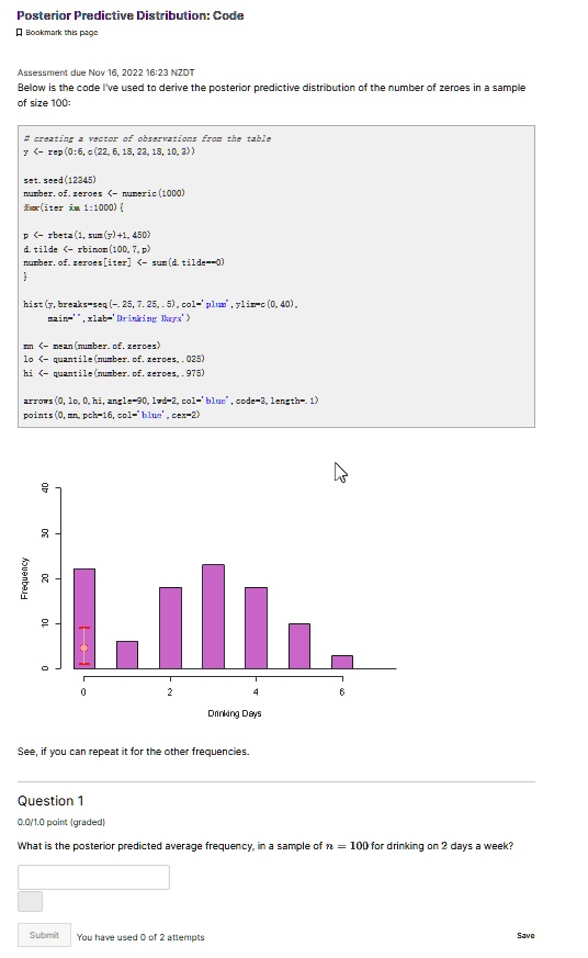
#creating a vector of observations from the table
y <- rep(0:6, c(22, 6, 18, 23, 18, 10, 3))
set.seed(12345)
number.of.zeroes <- numeric(1000)
for(iter in 1:1000) {
p <- rbeta(1, sum(y) + 1, 450)
d.tilde <- rbinom(100, 7, p)
number.of.zeroes[iter] <- sum(d.tilde == 0)
}
hist(y, breaks = seq(-.25, 7.25, .5), col = "plum", ylim = c(0, 40),
main = "", xlab = "Drinking Days")
mm <- mean(number.of.zeroes)
lo <- quantile(number.of.zeroes, .025)
hi <- quantile(number.of.zeroes, .975)
arrows(0, lo, 0, hi, angle = 90, lwd = 2, col = "blue", code = 3, length = .1)
points(0, mm, pch = 16, col = "blue", cex = 2)
See, if you can repeat it for the other frequencies.
Question 1
0.0/1.0 point (graded)
What is the posterior predicted average frequency, in a sample of $n = 100$ for drinking on 2 days a week?