Numerade

Questions asked

BEST MATCH

What is the maximal length of a codeword possible in a Huffman encoding of an alphabet of n symbols? Group of answer choices logn n/2 n-1 n

View Answer

BEST MATCH

When you hang a 100 g mass from a spring, the spring stretches 2 cm. If you remove the 100 g mass and hang another object of unknown mass, the spring stretches 6 cm. What is the mass of the object? (Assume the spring obeys Hooke’s law and doesn’t stretches beyond its elastic limit).

View Answer

BEST MATCH

8. Replace the circuit between A and B with a voltage source in series with a single resistor using source transformation.

View Answer

BEST MATCH

The monthly sales of a tuck shop decreased by $ 25 \% $ from two months ago to last month and increased by $ 18 \% $ from last month to this month. If the monthly sales this month is $ \$ 7292.4 $, find the monthly sales two months ago.

View Answer

BEST MATCH

What goes in blank B? Movies Total Utility (TU) Marginal Utility (MU) 0 0 A 1 30 B 2 55 C

View Answer

BEST MATCH

can automated OSINT tools balance the need for efficient data collection with the accuracy of reliability of the information? How might this be achieved?

View Answer

BEST MATCH

When the government imposes a magazine tax of $0.10 per magazine on buyers, the tax reduces the\\ for buyers. Now, buyers are willing to buy a given quantity of magazines only if the sale price before tax is\\ prices; similar to the price without a magazine tax prices; lower by $0.10 per magazine marginal benefits; similar to the price without a magazine tax marginal benefits; lower by $0.10 per magazine

View Answer

BEST MATCH

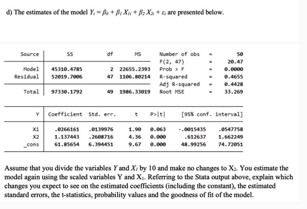
d) The estimates of the model Y_(i)=eta _(0)+eta _(1)x_(1i)+eta _(2)x_(2i)+epsi _(i) are presented below. Assume that you divide the variables Y and x_(l) by 10 and make no changes to x_(2). You estimate the model again using the scaled variables Y and x_(1). Referring to the Stata output above, explain which changes you expect to see on the estimated coefficients (including the constant), the estimated standard errors, the t-statistics, probability values and the goodness of fit of the model. d) The estimates of the model Y; = o + X + Xi + &; are presented below. Source ss dp MS Number of obs F(2,47) Prob > F R-squared Adj R-squared Root MSE 50 20.47 0.0000 0.4655 0.4428 33.269 = Model Residual 45310.4785 52019.7006 2 22655.2393 47 1106.80214 Total 97330.1792 49 1986.33019 Y Coefficient Std.err. t P>|t| [95% conf.interval] X1 X2 _cons .0266161 1.137443 61.85654 .0139976 .2608716 6.394451 1.90 4.36 9.67 0.063 0.000 0.000 -.0015435 .612637 48.99256 .0547758 1.662249 74.72051 Assume that you divide the variables Y and X by 10 and make no changes to X2. You estimate the model again using the scaled variables Y and X.. Referring to the Stata output above, explain which changes you expect to see on the estimated coefficients (including the constant), the estimated standard errors, the t-statistics, probability values and the goodness of fit of the model.

View Answer

BEST MATCH

If a rock is thrown vertically upward from the surface of Mars with velocity of 20 m/s, its height (in meters) after t seconds is $h = 20t - 1.86t^2$. (a) What is the velocity (in m/s) of the rock after 1 s? 16.28 m/s (b) What is the velocity (in m/s) of the rock when its height is 15 m on its way up? On its way down? (Round your answers to two decimal places.) up -8.07 m/s down m/s

View Answer

BEST MATCH

2. Consider a system which is initially in the state $\begin{pmatrix} 4-i \\ -2+5i \\ 3+2i \end{pmatrix}$ and having a Hamiltonian given by $\hat{H} = \frac{1}{\sqrt{2}} \begin{bmatrix} 0 & -i & 0 \\ i & 3 & 3 \\ 0 & 3 & 0 \end{bmatrix}$ (a) What condition must $\hat{H}$ satisfy? (b) If a measurement of $\hat{H}$ is carried out, what values will we obtain and with what probabilities? (c) Find the state of the system at a later time t. (d) Find the total energy of the system at t = 0 and any late time t by matrix algebra. Are these values different?

View Answer

jorge s.