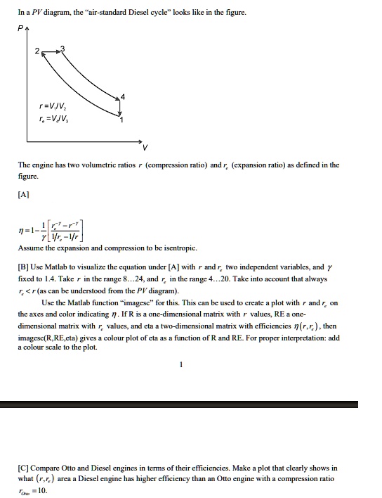
In a PV diagram, the "air-standard Diesel cycle" looks like in the figure.
PA
2
3
r = V$_2$/V$_1$
r$_c$ = V$_4$/V$_1$
4
1
V
The engine has two volumetric ratios r (compression ratio) and r$_c$ (expansion ratio) as defined in the
figure.
[A]
$\eta = 1 - \frac{1}{r^{\gamma - 1}} \left[ \frac{r_c^\gamma - r^\gamma}{\gamma (r_c - r)} \right]$
Assume the expansion and compression to be isentropic.
[B] Use Matlab to visualize the equation under [A] with r and r$_c$ two independent variables, and $\gamma$
fixed to 1.4. Take r in the range 8...24, and r$_c$ in the range 4...20. Take into account that always
r < r$_c$ (as can be understood from the PV diagram).
Use the Matlab function "imagesc" for this. This can be used to create a plot with r and r$_c$ on
the axes and color indicating $\eta$. If R is a one-dimensional matrix with r values, RE a one-
dimensional matrix with r$_c$ values, and eta a two-dimensional matrix with efficiencies $\eta$(r,r$_c$), then
imagesc(R,RE,eta) gives a colour plot of eta as a function of R and RE. For proper interpretation: add
a colour scale to the plot.
1
[C] Compare Otto and Diesel engines in terms of their efficiencies. Make a plot that clearly shows in
what (r,r$_c$) area a Diesel engine has higher efficiency than an Otto engine with a compression ratio
$\Gamma_{Otto} = 10.$