Numerade

Questions asked

BEST MATCH

1. A teacher is interested in studying the relationship between the average time studied in hours per week (X) and the grade of her students (Y) in their final examination. The students' grades and time studied are the following. Student# Hours Grade 1 5 92 2 3 77 3 2 84 4 0 64 5 5 80 6 4 99 7 1 72 8 3 83 9 8 95 10 2 87 The teacher knows a little bit of econometrics and is considering estimating the following regression model $Y_i = \beta_0 + \beta_1 X_i + u_i$. The notation is standard (as in this class), where $\bar{x}$ is the sample mean value of the $x$'s, $\hat{y}_i$ is the predicted value of the dependent variable (conditional on $x_i$) and $\hat{u}_i$ are the estimated residuals from the regression. a) Compute the OLS estimates for $\beta_0$ and $\beta_1$ (full credit requires showing of your calculations by hand or in Excel. Reporting only the estimated values is not enough)

View Answer

BEST MATCH

Sweet Management System Designing a comprehensive Sweet Management System requires careful consideration of various aspects to ensure it meets the needs of users. Below is a detailed list of requirements for the Sweet Management System. Requirements for Sweet Management System Admin Requirements 1. User Management  Manage user accounts including store owners and raw material suppliers. 2. Monitoring and Reporting  Monitor profits and generate financial reports.  Identify best-selling products in each store.  Gather and display statistics on registered users by City (Nablus/Jenin etc...) 3. Content Management  Manage the content shared on the system, including recipes and posts.  Manage user feedback. Store Owners and Raw Material Suppliers Requirements 1. Product Management  Add, update, and remove available products.  Monitor sales and profits.  Identify best-selling products.  Implement dynamic discount features. 2. Communication and Notification  Use the messaging system to communicate with users and other suppliers.  Receive notifications [via email] for special requests. [OPTIONAL /BONUS] 3. Account Management  Manage account details and update business information. 4. Order Management  Process and track orders [status]. Beneficiary Users Requirements 1. User Account  Sign up for a new account.  Sign in to the platform.  Manage personal accounts.  Post and share personal dessert creations. 2. Exploration and Purchase  Browse and search for dessert recipes.  Filter recipes based on dietary needs or food allergies.  Purchase desserts directly from store owners. 3. Communication and Feedback  Directly communicate with store owners and suppliers for inquiries or assistance.  Provide feedback on purchased products and shared recipes.

View Answer

BEST MATCH

During which stage did American psychology begin to emphasize individual differences, adaptation to the environment, and practicality? Stage One: Moral and mental philosophy Stage Two: Intellectual philosophy Stage Three: The U.S. Renaissance Stage Four : U.S. functionalism

View Answer

BEST MATCH

11. (4 points) Let X be the set of all bounded sequences of real numbers. Define $d(x, y) = \sup_{n \in \mathbb{N}} |x_n - y_n|$ for all $x = (x_n), y = (y_n) \in X$. 11.1. Show that $d$ is a metric on X. 11.2. Let $z = (\frac{1}{n}) \in X$. Give an example of a Cauchy sequence in $B_d(z; 1)$ which is not convergent in $B_d(z; 1)$.

View Answer

BEST MATCH

The illustration above represents a G protein-coupled receptor. Question 44 Select one: a. True b. False

View Answer

BEST MATCH

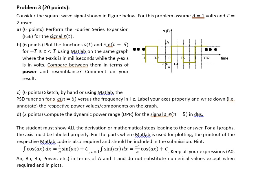
Texts: For all problems, final answers without detailed work do not count. Partial marks are allocated for intermediate steps/calculations. Problem 3 (20 points): Consider the square-wave signal shown in Figure below. For this problem, assume A = 1 volts and T = 2 msec. a) (6 points) Perform the Fourier Series Expansion (FSE) for the signal s(t). s(t) b) (6 points) Plot the functions s(t) and s_e(n=5) for -T < t < T using Matlab on the same graph, where the t-axis is in milliseconds and the y-axis is in volts. Compare them in terms of power and resemblance. Comment on your result. T/2 3T/2 time c) (6 points) Sketch, by hand or using Matlab, the PSD function for s_e(n=5) versus the frequency in Hz. Label your axes properly and write down (i.e. annotate) the respective power values/components on the graph. d) (2 points) Compute the dynamic power range (DPR) for the signal s_e(n=5) in dBs. The student must show ALL the derivation or mathematical steps leading to the answer. For all graphs, the axes must be labeled properly. For the parts where Matlab is used for plotting, the printout of the respective Matlab code is also required and should be included in the submission. Hint: Express all variables (An, Bn, Power, etc.) in terms of A and T and do not substitute numerical values except when required and in plots.

View Answer

BEST MATCH

Texts: The amount of water to be carried by a canal excavated in a concrete channel (n=0.013) is 4 m^3/s. It has side slopes of 2H:1V and a bed slope of 400 mm/km. a) If the depth of flow is to be 1.25 m, what must be the bottom width to carry the discharge? What is the flow area? b) How does your answer in (a) above compare with the depth and bottom width for the most efficient trapezoidal section (z = 1/√3)? Please solve.

View Answer

BEST MATCH

Nitrobenzene is a very important industrial chemical. Most of the nitrobenzene produced in the United States is used to manufacture a chemical called aniline. Nitrobenzene is also used to produce lubricating oils such as those used in motors and machinery. Mostly, nitrobenzene is produced by the reaction of benzene with nitric acid, which is highly exothermic and uses H2SO4 as a catalyst, which tends to be corrosive. So, in order to avoid this problem, a less corrosive reaction employs NO2 as the nitrating agent as illustrated below: NO2 NO HO A + 2B 2C + D If this liquid phase reaction is carried out in an adiabatic CSTR, what will be the reactor volume and residence time necessary to achieve 65% conversion of NO2? Also, the reaction is first order with respect to A and second order with respect to B. Hrx = 370.1 * 10^3 J/mol T = 303 K molÂ·J Cp = 84.5 molÂ·K Cpg = 137 molÂ·K Cpc = 170 molÂ·K Cpp = 75 molÂ·K molÂ·mol FAo = 10 mol/min Fo = 30 mol/min k(303 K) = 0.09 min^-1 E = 40,000 J/mol mol! Lv = 100 min C = 0.01 mol/LÂ·min

View Answer

BEST MATCH

what is the side effects of good health and well being?

View Answer

BEST MATCH

Though my neighbor's drone crashed into the side of my house, it was not damaged.

View Answer

lindsay p.