PROBLEM 1: Diffusion equation - Matlab Intensive
Imagine a 1D rod that is L long. We will investigate two cases of boundary conditions:
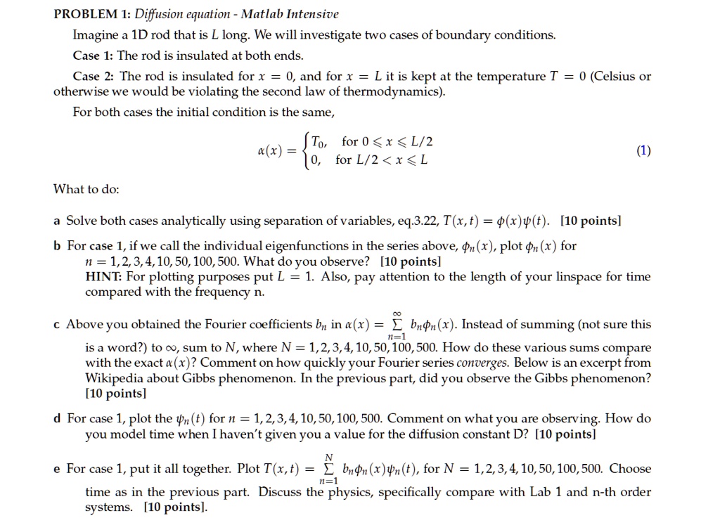
Case 1: The rod is insulated at both ends.
Case 2: The rod is insulated for x = 0, and for x = L it is kept at the temperature T = 0 (Celsius or otherwise we would be violating the second law of thermodynamics).
For both cases, the initial condition is the same:
T(x, t) =
0, for 0 < x < L/2
0, for L/2 < x < L
What to do:
a) Solve both cases analytically using separation of variables, eq.3.22, T(x, t) = (x)(t). [10 points]
b) For case 1, if we call the individual eigenfunctions in the series above, n(x), plot n(x) for n = 1, 2, 3, 4, 10, 50, 100, 500. What do you observe? [10 points] HINT: For plotting purposes, put L = 1. Also, pay attention to the length of your linspace for time compared with the frequency n.
c) Above, you obtained the Fourier coefficients b_n in (x) = b_n * n(x). Instead of summing (not sure this is a word?) to infinity, sum to N, where N = 1, 2, 3, 4, 10, 50, 100, 500. How do these various sums compare with the exact (x)? Comment on how quickly your Fourier series converges. Below is an excerpt from Wikipedia about Gibbs phenomenon. In the previous part, did you observe the Gibbs phenomenon? [10 points]
d) For case 1, plot n(t) for n = 1, 2, 3, 4, 10, 50, 100, 500. Comment on what you are observing. How do you model time when I haven't given you a value for the diffusion constant D? [10 points]
e) For case 1, put it all together. Plot T(x, t) = b_n * n(x) * n(t), for N = 1, 2, 3, 4, 10, 50, 100, 500. Choose time as in the previous part. Discuss the physics, specifically compare with Lab 1 and n-th order systems. [10 points].