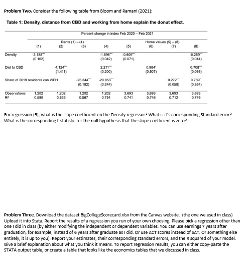
Problem Two. Consider the following table from Bloom and Ramani (2021):
Table 1: Density, distance from CBD, and working from home explain the donut effect.
Percent change in index Feb 2020 Feb 2021 Rents (1) (4) (g) (s) son(ea ewoH (1) (2) (3) (4) (s) (6) (7) Density -3.188** -1.596** -0.609** (0.162) (0.042) (0.071) Dist to CBD 4.124** 2.211** 0.984* (1.411) (0.200) (0.507) Share of 2019 residents can WFH -25.344** -20.853** 0.272** (0.244) (0.058) 1,202 1,202 1,202 1,202 3,693 3,693 3,693 R2 0.580 0.625 0.567 0.734 0.741 0.746 0.712
(8) -0.259' (0.044) 0.708** (990'0) 0.769* (1190)
3,693 0.749
What is the corresponding t-statistic for the null hypothesis that the slope coefficient is zero?
Problem Three. Download the dataset BigCollege5corecard.xlsx from the Canvas website (the one we used in class). Upload it into Stata. Report the results of a regression you run of your own choosing. Please pick a regression other than one I did in class (by either modifying the independent or dependent variables). You can use earnings 7 years after graduation, for example, instead of 6 years after graduation as I did. Or use ACT scores instead of SAT. Or something else entirely, it is up to you. Report your estimates, their corresponding standard errors, and the R squared of your model.
STATA output table, or create a table that looks like the economics tables that we discussed in class.