Project Assignment: Tank System Simulation
Objective
Simulate the dynamics of an interconnected tank system using Simulink and
MATLAB ODE code. This project aims to provide hands-on experience in
modeling and simulating a system with two interconnected tanks.
Equations
The dynamics of the tank levels and {:h_(2)) can be described by the following
differential equations:
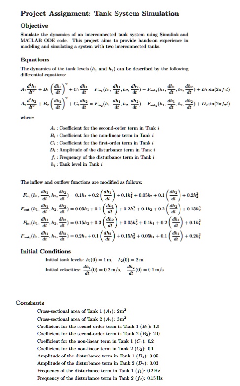
A_(1)(d^(2)h_(1))/(dt^(2))+B_(1)((dh_(1))/(dt))^(2)+C_(1)(dh_(1))/(dt)=F_(in_(1))(h_(1),(dh_(1))/(dt),h_(2),(dh_(2))/(dt))-F_(aut_(1))(h_(1),(dh_(1))/(dt),h_(2),(dh_(2))/(dt))+D_(1)sin(2pi f_(1)t)
A_(2)(d^(2)h_(2))/(dt^(2))+B_(2)((dh_(2))/(dt))^(2)+C_(2)(dh_(2))/(dt)=F_(in_(2))(h_(1),(dh_(1))/(dt),h_(2),(dh_(2))/(dt))-F_(aut_(2))(h_(1),(dh_(1))/(dt),h_(2),(dh_(2))/(dt))+D_(2)sin(2pi f_(2)t)
where:
A_(i): Coefficient for the second-order term in Tank i
B_(i) : Coefficient for the non-linear term in Tank i
C_(i): Coefficient for the finst-order term in Tank i
D_(i) : Amplitude of the disturbance term in Tank i
f_(i) : Frequency of the disturbance term in Tank i
h_(i)= Tank level in Tank i
The inflow and outflow functions are modified as follows:
F_(in )(h_(1),(dh_(1))/(dt),h_(2),(dh_(2))/(dt))=0.1h_(1)+0.2((dh_(1))/(dt))+0.1h_(1)^(2)+0.05h_(2)+0.1((dh_(2))/(dt))+0.2h_(2)^(2)
F_(out )(h_(1),(dh_(1))/(dt),h_(2),(dh_(2))/(dt))=0.05h_(1)+0.1((dh_(1))/(dt))+0.2h_(1)^(2)+0.1h_(2)+0.2((dh_(2))/(dt))+0.15h_(2)^(2)
F_(in )(h_(1),(dh_(1))/(dt),h_(2),(dh_(2))/(dt))=0.15h_(2)+0.3((dh_(2))/(dt))+0.05h_(2)^(2)+0.1h_(1)+0.2((dh_(1))/(dt))+0.1h_(1)^(2)
F_(eut )(h_(1),(dh_(1))/(dt),h_(2),(dh_(2))/(dt))=0.2h_(2)+0.1((dh_(2))/(dt))+0.15h_(2)^(2)+0.05h_(1)+0.1((dh_(1))/(dt))+0.2h_(1)^(2)
Initial Conditions
Initial tank levels: h_(1)(0)=1m,h_(2)(0)=2m
Initial velocities: (dh_(1))/(dt)(0)=0.2(m)/(s),(dh_(2))/(dt)(0)=0.1(m)/(s)
Constants
Croes-sectional area of Tank 1(A_(1)):2m^(2)
Cross-sectional area of Tank 2(A_(2)):3m^(2)
Coefficient for the second-order term in Tank 1(B_(1)):1.5
Coefficient for the second-order term in Tank 2 ( {:B_(2)):2.0
Coefficient for the non-linear term in Tank 1(C_(1)):0.2
Coefficient for the non-linear term in Tank 2(C_(2)):0.1
Amplitude of the disturbance term in Tank 1(D_(1)):0.05
Amplitude of the disturbance term in Tank 2(D_(2)):0.03
Frequency of the disturbance term in Tank 1(f_(1)):0.2Hz
Frequency of the disturbance term in Tank 2(f_(2)):0.15Hz
Project Assignment: Tank System Simulation
Objective
Simulate the dynamics of an interconnected tank system using Simulink and MATLAB ODE code. This project aims to provide hands-on experience in modeling and simulating a system with two interconnected tanks.
Equations The dynamics of the tank levels (h, and h2) can be described by the following differential equations:
A+(+c=Fm.h-Fm.h+Dsnt T
where:
A; : Coefficient for the second-order term in Tank i B; : Coefficient for the non-linear term in Tank i C; : Coefficient for the first-order term in Tank i D; : Amplitude of the disturbance term in Tank i fi : Frequency of the disturbance term in Tank i h; : Tank level in Tank i
The infiow and outflow functions are modified as follows:
Finm.h.=0.1h+0.2+0.1h+0.05h+0.1+0.2h
Fom.h.2=0.2h+0.+0.15h+0.o5h+0.+0.2h Initial Conditions Initial tank levels: h1(0) = 1 m, h2(0) = 2 m
Initial velocities: dt
dt
Constants Cross-sectional area of Tank 1 (A1): 2 m2 Cross-sectional area of Tank 2 (A2): 3 m2 Coefficient for the second-order term in Tank 1 (B): 1.5 Coefficient for the second-order term in Tank 2 (B): 2.0 Coefficient for the non-linear term in Tank 1 (C1): 0.2 Coefficient for the non-linear term in Tank 2 (C2): 0.1 Amplitude of the disturbance term in Tank 1 (Di): 0.05 Amplitude of the disturbance term in Tank 2 (D2): 0.03 Frequency of the disturbance term in Tank 1 (f1): 0.2 Hz Frequency of the disturbance term in Tank 2 (f2): 0.15 Hz