Numerade

Questions asked

BEST MATCH

Lower-income women are more likely to be obese than higher income women. True False

BEST MATCH

Suppose we have three unity-magnitude complex numbers whose phase angles are $\pi/4$ radians, $-3\pi/4$ radians, and $-\pi/4$ radians. What is the average phase angle of the three phase angles? Show your work.

View Answer

BEST MATCH

3. (0.2 pts) Arrange the gametes from mother and father (problem 2) into a Punnett square format (hint 1: only need a |*1 Punnett Square (not a 2 * 2 ). ( Hint 2: You should notice that the genotype results in a phenotype of all kittens having black fur and curled ears .)

View Answer

BEST MATCH

[TRUE / FALSE] A player's mixed strategy Nash equilibrium strategy can involve putting positive probability on strictly dominated strategies.

View Answer

BEST MATCH

how long would it take you to get 50,000 points if you get 10 points every 5 minutes

View Answer

BEST MATCH

3. Two polymer blocks shown in figure are bonded to a rigid support mount and to a movable plate (1). The polymer block has a Young's modulus E=10 GPa and Poisson's ratio 0.45. When a force P = 1,600 N is applied to the assembly, determine the horizontal deflection of plate (1).

View Answer

BEST MATCH

The quotient of $3\frac{1}{5}$ and $2\frac{1}{3}$

View Answer

BEST MATCH

4. Make function machines with 4 input and 4 output values using the given rules below: a. Subtract 10 from the input value b. Multiply the input by 3 c. Multiply the input by 2 and then add 5 d. Add 5 to the input and then multiply by 2 e. Are the output values for question (c) and (d) the same? f. Does it make a difference whether we first add and then multiply or first multiply and 5. Find the rule for calculating the output value for every given input value in th

View Answer

BEST MATCH

Problem (6) [10 points] What is the output of this code? class A { private: int x; int y; public: virtual void foo(); A(); }; class B : public A { private: int x; public: void foo(); B(); }; class C : public A { private: int x; public: void foo(); C(); }; A::A() { cout << "Heya!\n"; x=1; } B::B() { x=2; } C::C() { cout << "Live long and prosper\n"; x=3; } void A::foo() { cout << x << endl; } void B::foo() { cout << x << endl; } int main() { C d; B s; s.foo(); // B object d.foo(); // C object }

View Answer

BEST MATCH

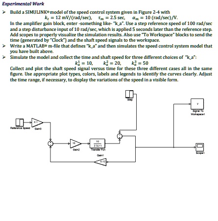
Experimental Work Build a SIMULINK® model of the speed control system given in Figure 2-4 with k_a = 12 mV/(rad/sec), $T_m = 2.5$ sec, $a_m = 10$ (rad/sec)/V. In the amplifier gain block, enter -something like- "k_a". Use a step reference speed of 100 rad/sec and a step disturbance input of 10 rad/sec, which is applied 5 seconds later than the reference step. Add scopes to properly visualize the simulation results. Also use "To Workspace" blocks to send the time (generated by "Clock") and the shaft speed signals to the workspace. Write a MATLAB® m-file that defines "k_a" and then simulates the speed control system model that you have built above. Simulate the model and collect the time and shaft speed for three different choices of "k_a": k_a = 10, k_a = 20, k_a = 50 Collect and plot the shaft speed signal versus time for these three different cases all in the same figure. Use appropriate plot types, colors, labels and legends to identify the curves clearly. Adjust the time range, if necessary, to display the variations of the speed in a visible form.

View Answer

miguel c.