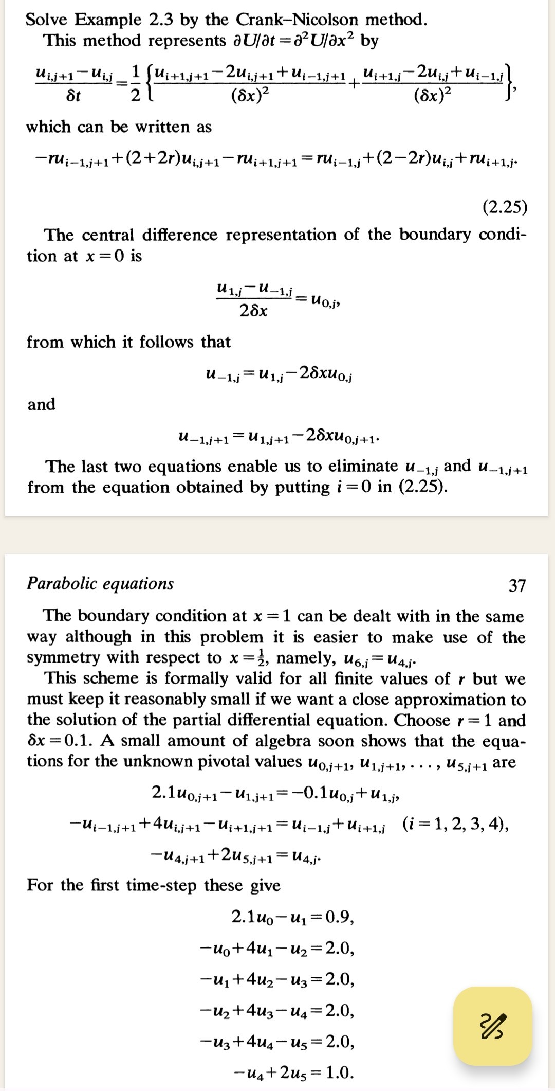
Solve Example 2.3 by the Crank-Nicolson method.
This method represents \( \partial U / \partial t=\partial^{2} U / \partial x^{2} \) by
\[
\frac{u_{i, j+1}-u_{i, j}}{\delta t}=\frac{1}{2}\left\{\frac{u_{i+1, j+1}-2 u_{i, j+1}+u_{i-1, j+1}}{(\delta x)^{2}}+\frac{u_{i+1, j}-2 u_{i, j}+u_{i-1, j}}{(\delta x)^{2}}\right\},
\]
which can be written as
\[
-r u_{i-1, j+1}+(2+2 r) u_{i, j+1}-r u_{i+1, j+1}=r u_{i-1, j}+(2-2 r) u_{i, j}+r u_{i+1, j}
\]
The central difference representation of the boundary condition at \( x=0 \) is
\[
\frac{u_{1, j}-u_{-1, j}}{2 \delta x}=u_{0, j}
\]
from which it follows that
\[
u_{-1, j}=u_{1, j}-2 \delta x u_{0, j}
\]
and
\[
u_{-1, j+1}=u_{1, j+1}-2 \delta x u_{0, j+1} .
\]
The last two equations enable us to eliminate \( \boldsymbol{u}_{-1, j} \) and \( \boldsymbol{u}_{-1, i+1} \) from the equation obtained by putting \( i=0 \) in (2.25).
Parabolic equations
37
The boundary condition at \( x=1 \) can be dealt with in the same way although in this problem it is easier to make use of the symmetry with respect to \( x=\frac{1}{2} \), namely, \( u_{6, j}=u_{4, j} \).
This scheme is formally valid for all finite values of \( r \) but we must keep it reasonably small if we want a close approximation to the solution of the partial differential equation. Choose \( r=1 \) and \( \delta x=0.1 \). A small amount of algebra soon shows that the equations for the unknown pivotal values \( u_{0, j+1}, u_{1, j+1}, \ldots, u_{5, j+1} \) are
\[
\begin{aligned}
2.1 u_{0, j+1}-u_{1, j+1} & =-0.1 u_{0, j}+u_{1, j}, \\
-u_{i-1, j+1}+4 u_{i, j+1}-u_{i+1, j+1} & =u_{i-1, j}+u_{i+1, j} \quad(i=1,2,3,4), \\
-u_{4, j+1}+2 u_{5, j+1} & =u_{4, j} .
\end{aligned}
\]
For the first time-step these give
\[
\begin{aligned}
2.1 u_{0}-u_{1} & =0.9 \\
-u_{0}+4 u_{1}-u_{2} & =2.0 \\
-u_{1}+4 u_{2}-u_{3} & =2.0 \\
-u_{2}+4 u_{3}-u_{4} & =2.0 \\
-u_{3}+4 u_{4}-u_{5} & =2.0 \\
-u_{4}+2 u_{5} & =1.0
\end{aligned}
\]