Just need help 3 & 4 please!!
Type this code into Python and verify that it generates samples of the signal b_(3)(t). Make two plots of the signal you generated: one should be a line plot versus time t (in seconds, stored in vector tt3) and the other should be a stem plot versus the discrete index n (stored in vector n3).
Using the code described above as a model, write code to generate samples of the length 7 and length 13 Barker codes. Use the same sample period (0.01) that you used to generate the length 3 codes. Include plots of the signals b_(7)(t) and b_(13)(t) in your report.
2.3 Implementing matched filters for Barker codes
The matched filter for the signal b[n] is defined as h_(MF)(t) = b[-n]. For the Barker codes above, b[n] was non-zero for n >= 0, thus it is easy to see that h_(MF)[n] will not be zero for n <= 0. This means that the matched filter will not be a causal system. Because b[n] has a finite length, we can fix this problem by delaying h_(MF)[n] enough to make it causal. This new causal version of the matched filter is defined as h_(MFC) = h_(MF)[n - n_(c)].
For each of the 3 Barker codes, and {b_(13)}, determine the value for n_(c) required to make their matched filters causal. Suppose that we apply a causal matched filter to a signal. How is the result related to the autocorrelation? In other words, if we compute phi_(causal)[n] = b[n] ** h_(MFC)[n], how is phi_(causal)[n] related to phi[n]?
In Python, it is easy to generate the causal matched filter for a given signal. You can flip the data in the Barker code vector around to create the samples needed for the matched filter. For example, the code below creates the matched filter for the length 3 Barker sequence:
hmf3 = b3[::-1]
Use this or a similar command to generate the causal matched filters for the 3 Barker code signals. Plot the matched filters versus time and include the plots in your report. Note that you will have to define a time vector to plot your Barker code against.
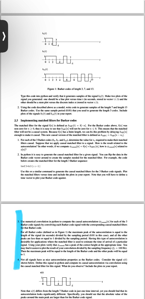
Use numerical convolution in Python to compute the causal autocorrelation (phi_(causal)[n] for each of the 3 Barker code signals by convolving each Barker code signal with the corresponding causal matched filters for that Barker code.
For all Barker codes (defined as in Figure 1), the maximum peak of the autocorrelation is equal to the length of the signal (in seconds) divided by the sampling period (0.01 in this case), and all the other peaks are less than or equal to 1 divided by the sampling period. Having this type of autocorrelation is desirable for applications where the matched filter is used to estimate the time of arrival of a particular signal. Using your plots verify that phi_(causal) has a peak of the correct height at the appropriate time. You may find it easiest to plot the result of your convolution divided by the sampling frequency (f).
Then the maximum peak will be equal to the length of the Barker code and the other peaks will be equal to 1.
Not all signals have as nice autocorrelation properties as the Barker codes. Consider the signal s(t) shown below. Define this signal in Python and compute its causal autocorrelation via convolution using the causal matched filter for this signal. What do you observe? Include the plots in your report.
bs(f)
br(t)
bia(t)
Figure 1: Barker codes of length 3, 7, and 13.
Type this code into Python and verify that it generates samples of the signal bs(e). Make two plots of the signal you generated: one should be a line plot versus time t (in seconds, stored in vector tt3) and the other should be a stem plot versus the discrete index n (stored in vector n3).
2. Using the code described above as a model, write code to generate samples of the length 7 and length 13 Barker codes. Use the same sample period (0.01) that you used to generate the length 3 codes. Include plots of the signals br(t) and b13(t) in your report.
2.3 Implementing matched filters for Barker codes
The matched filter for the signal 6[] is defined as AMF(t) = b[n], For the Barker codes above, b[] was non-zero for n >= 0, thus it is easy to see that hsp[n] will not be zero for n >= 0. This means that the matched filter will not be a causal system. Because b[n] has a finite length, we can fix this problem by delaying hMF[n] enough to make it causal. This new causal version of the matched filter is defined as hypc = hyer[n - ne]. I. For each of the 3 Barker codes (b, b, and bs), determine the value for required to make their matched filters causal. Suppose that we apply a causal matched filter to a signal. How is the result related to the autocorrelation? In other words, if we compute caual[n] = b[n] - hypc[n], how is (causal[n] related to o[n]? 2. In Python it is easy to generate the causal matched filter for a given signal. You can flip the data in the Barker code vector around to create the samples needed for the matched filter. For example, the code below creates the matched filter for the length 3 Barker sequence:
hmf3 = b3[::-1]
Use this or a similar command to generate the causal matched filters for the 3 Barker code signals. Plot the matched filters versus time and include the plots in your report. Note that you will have to define a time vector to plot your Barker code against.
3. Use numerical convolution in Python to compute the causal autocorrelation (caual[n] for each of the 3 Barker code signals by convolving each Barker code signal with the corresponding causal matched filters for that Barker code. For all Barker codes (defined as in Figure 1), the maximum peak of the autocorrelation is equal to the length of the signal (in seconds) divided by the sampling period (0.01 in this case), and all the other peaks are less than or equal to 1 divided by the sampling period. Having this type of autocorrelation is desirable for applications where the matched filter is used to estimate the time of arrival of a particular nsedodeyeseeasd ne may find it easiest to plot the result of your convolution divided by the sampling frequency f=100Hz Then the maximum peak will be equal to the length of the Barker code and the other peaks will be equal to 1.
4. Not all signals have as nice autocorrelation properties as the Barker codes. Consider the signal s(t) shown below. Define this signal in Python and compute its causal autocorrelation via convolution using the causal matched filter for this signal. What do you observe? Include the plots in your report.
s(t)
Note that s(t) differs from the length 7 Barker code in just one time interval, yet you should find that its autocorrelation looks significantly different. Specifically, you should see that the absolute value of the peaks around the main peak are larger than for the Barker code signal.