Place a control button in the worksheet that calls a VBA macro that processes the following
sales data (your final code should work with data sheets that have more or fewer regions and
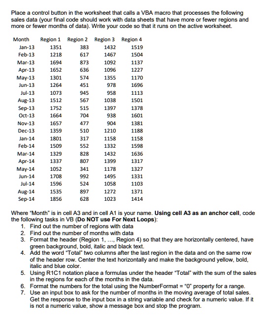
more or fewer months of data). Write your code so that it runs on the active worksheet.
Where "Month" is in cell A3 and in cell A1 is your name. Using cell A3 as an anchor cell, code
the following tasks in VB (Do NOT use For Next Loops):
Find out the number of regions with data
Find out the number of months with data
Format the header (Region 1,..., Region 4) so that they are horizontally centered, have
green background, bold, italic and black text.
Add the word "Total" two columns after the last region in the data and on the same row
of the header row. Center the text horizontally and make the background yellow, bold,
italic and blue color.
Using R1C1 notation place a formulas under the header "Total" with the sum of the sales
in the regions for each of the months in the data.
Format the numbers for the total using the NumberFormat = " 0 " property for a range.
Use an input box to ask for the number of months in the moving average of total sales.
Get the response to the input box in a string variable and check for a numeric value. If it
is not a numeric value, show a message box and stop the program.
If the user enters a
valid number but it cannot be used because it exceeds the number of months available
to calculate an average, then show a message box stating “Number in Moving Average
is ##. This number cannot be greater than ##” and stop the program.
8. Clear the column where the moving averages of total sales are going to be. That is, clear
the column that is three columns to the right of the last column with the sales data. (A
moving average is the average of the previous months. For example, if the moving
average is for 3 months, the first moving average that can be calculated is for the 4-th
month and is equal to the average of the previous three months. The average of the 2nd,
3rd and 4th months is the moving average for the 5-th month, etc.) Note that the last
moving average is the predicted sales for one month after the last month with data (Oct-
14 in this example).
9. If the number of months in the moving average specified in the input box is less than or
equal to the number of months of data then use the fromulaR1C1 property to calculate
the moving average corresponding to the first month where the moving average can be
calculated (i.e., if number of months in the moving average is 4, then the first month for
which the moving average can be calculated is month 5). Then copy this equation to all
subsequent months until one month past the last month in the data. (Alternatively, you
can specify the formulaR1C1 property to all the months that will have a calculated
moving average.)
10. Format the numbers for the moving averages using the NumberFormat = “0.00” property
for a range.
11. Label this column “Moving Average (#)” where # is the number of months in the moving
average specified in the input box. Format this header with left-justified horizontal
alignment, blue, bold and italic text.
12. In column A, label the row that is two rows after the last row of data with the word “Avg”.
Center the text horizontally, make the font bold, italic and blue color and background
yellow.
13. Using a string address extracted from a range defined using Range(Range(),
Range()).Address to construct a formula to calculate the average over all months for
Region 1 and place it under the column for Region 1 and on the same row where the
word “Avg” was entered. Copy the cell with formula to calculate the average for the first
region to the other three regions. (Note: if you prefer doing steps 13 a different way, it is
ok.)
14. Format the numbers for the averages using the NumberFormat = “0.00” property for a
range.
For your records print the VB code using the task descriptions above as comments to your
code to document the code. Add a worksheet named “forms” with the following (where the
number in the moving average can be any valid number):
Input box used to ask for the number of months in the moving average and the two message
boxes. (use to place an image onto clipboard and then to paste or
alternatively you can use the “snipping tool”). The first line in your code should have “Option
Explicit” and your second line should be a comment statement with your name.
Place a control button in the worksheet that calls a VBA macro that processes the following sales data (your final code should work with data sheets that have more or fewer regions and more or fewer months of data). Write your code so that it runs on the active worksheet.
Month Region 1 Region 2 Region 3 Region 4 Jan-13 1351 383 1432 1519 Feb-13 1218 617 1467 1504 Mar-13 1694 873 1092 1137 Apr-13 1652 636 1096 1227 May-13 1301 574 1355 1170 Jun-13 1264 451 978 1696 Jul-13 1073 945 958 1113 Aug-13 1512 567 1038 1501 Sep-13 1752 515 1397 1378 Oct-13 1664 704 938 1601 Nov-13 1657 477 904 1381 Dec-13 1359 510 1210 1188 Jan-14 1801 317 1158 1158 Feb-14 1509 552 1332 1598 Mar-14 1329 828 1432 1636 Apr-14 1337 807 1399 1317 May-14 1052 341 1178 1327 Jun-14 1708 992 1495 1331 Jul-14 1596 524 1058 1103 Aug-14 1535 897 1272 1371 Sep-14 1856 628 1023 1414
Where Month is in cell A3 and in cell A1 is your name. Using cell A3 as an anchor cell, code the following tasks in VB (Do NOT use For Next Loops): 1. Find out the number of regions with data 2. Find out the number of months with data Format the header (Region 1, ..., Region 4) so that they are horizontally centered, have green background, bold, italic and black text. 4 Add the word Total two columns after the last region in the data and on the same row of the header row. Center the text horizontally and make the background yellow, bold, italic and blue color. Using R1C1 notation place a formulas under the header Total with the sum of the sales in the regions for each of the months in the data. 6. Format the numbers for the total using the NumberFormat = 0 property for a range. 7. Use an input box to ask for the number of months in the moving average of total sales. Get the response to the input box in a string variable and check for a numeric value. If it is not a numeric value, show a message box and stop the program.