Ace - AI Tutor
Ask Our Educators
Textbooks
My Library
Flashcards
Scribe - AI Notes
Notes & Exams
Download App
Sarah

Sarah

Divider

Questions asked

ANSWERED

Shu Naito verified

Numerade educator

For major league baseball teams, is there a relationship between player payrolls and gate money? Here are data for each of the American League teams for the year 2002. The variable x denotes the 2002 player payroll (in millions of dollars), and the variable y denotes the mean attendance (in thousands of fans) for the 81 home games that year. The data are plotted in the Figure 1 scatter plot. Also given is the product of the player payroll and the mean attendance for each of the fourteen teams. (These products, written in the column labelled "xy", may aid in calculations.) | | Player payroll, x (in $1,000,000s) | Mean attendance, y (in thousands) | xy | | :--- | :--- | :--- | :--- | | Anaheim | 62.8 | 28.52 | 1791.056 | | Baltimore | 56.5 | 33.09 | 1869.585 | | Boston | 110.2 | 32.72 | 3605.744 | | Chicago White Sox | 54.5 | 20.74 | 1130.33 | | Cleveland | 74.9 | 32.35 | 2423.015 | | Detroit | 54.4 | 18.52 | 1007.488 | | Kansas City | 49.4 | 16.30 | 805.22 | | Minnesota | 41.3 | 23.70 | 978.81 | | New York Yankees | 133.4 | 42.84 | 5714.856 | | Oakland | 41.9 | 26.79 | 1122.501 | | Seattle | 86.1 | 43.70 | 3762.57 | | Tampa Bay | 34.7 | 13.21 | 458.387 | | Texas | 106.9 | 29.01 | 3101.169 | | Toronto | 66.8 | 20.25 | 1352.7 | What is the slope of the least-squares regression line for these data? Carry your intermediate computations to at least four decimal places and round your answer to at least two decimal places. (If necessary, consult a list of formulas.)

View Answer
divider
ANSWERED

Manisha Sarker verified

Numerade educator

In ongoing economic analyses, the federal government compares per capita incomes not only among different states but also for the same state at different times. Typically, what the federal government finds is that "poor" states tend to stay poor and "wealthy" states tend to stay wealthy. Would we have gotten information about the 1999 per capita income for a state (denoted by y) from its 1980 per capita income (denoted by x)? The following bivariate data give the per capita income (in thousands of dollars) for a sample of fifteen states in the years 1980 and 1999 (source: U.S. Bureau of Economic Analysis, Survey of Current Business, May 2000). The data are plotted in the scatter plot in Figure 1. Also given is the product of the 1980 per capita income and the 1999 per capita income for each of the fifteen states. (These products, written in the column labelled "xy", may aid in calculations.) | | 1980 per capita income, x (in $1000s) | 1999 per capita income, y (in $1000s) | xy | | :--- | :---: | :---: | :---: | | Georgia | 8.5 | 27.2 | 231.2 | | North Dakota | 8.1 | 23.5 | 190.35 | | Michigan | 10.4 | 27.8 | 289.12 | | Hawaii | 11.5 | 27.8 | 319.7 | | North Carolina | 8.2 | 26.2 | 214.84 | | Oregon | 10.2 | 27.1 | 276.42 | | New Jersey | 11.8 | 36.1 | 425.98 | | California | 12.0 | 29.8 | 357.6 | | Ohio | 10.1 | 27.1 | 273.71 | | Louisiana | 8.8 | 22.8 | 200.64 | | Nevada | 11.8 | 30.4 | 358.72 | | South Dakota | 8.1 | 25.1 | 203.31 | | Montana | 9.1 | 22.3 | 202.93 | | Tennessee | 8.3 | 25.6 | 212.48 | | Idaho | 8.7 | 23.4 | 203.58 | What is the sample correlation coefficient for these data? Carry your intermediate computations to at least four decimal places and round your answer to at least three decimal places. (If necessary, consult a list of formulas.)

View Answer
divider
ANSWERED

Manisha Sarker verified

Numerade educator

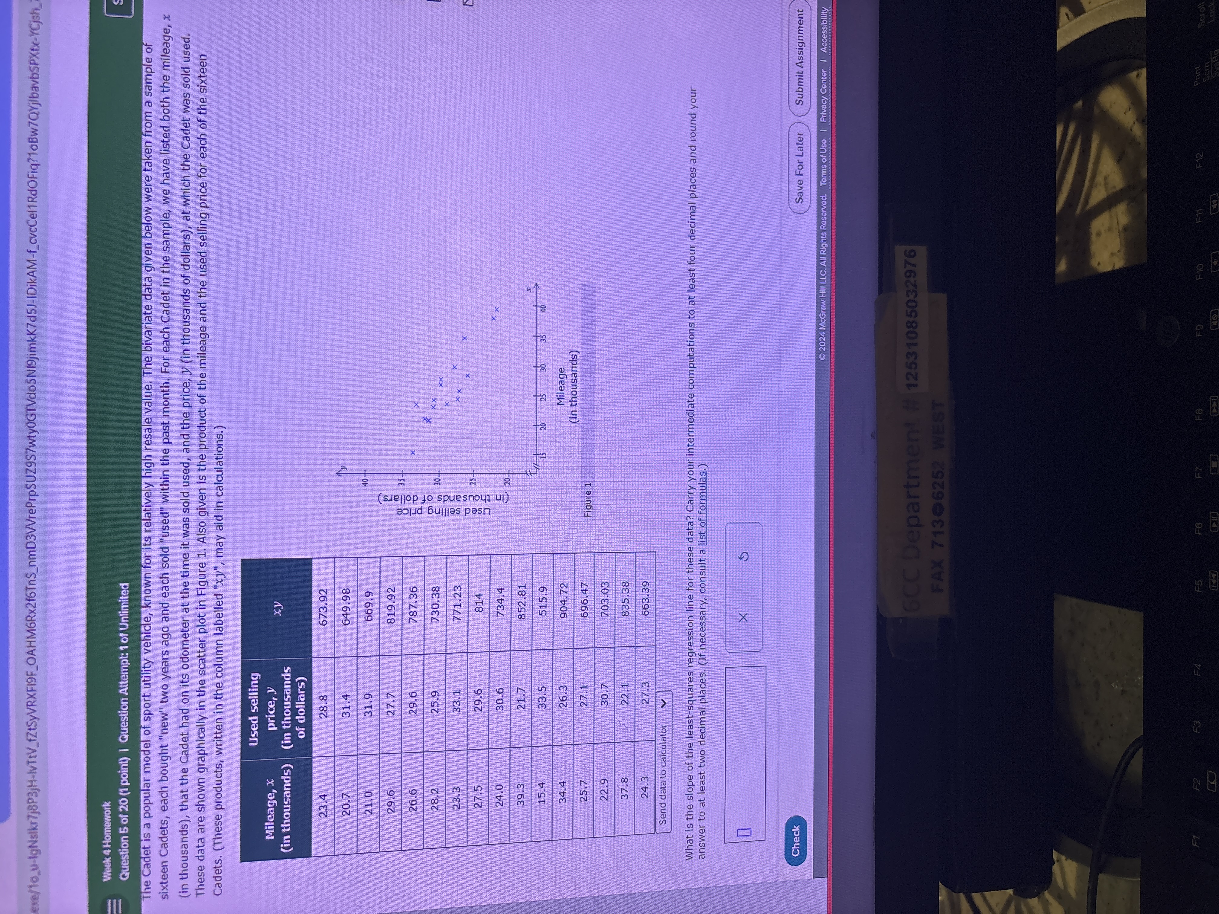
Week 4 Homework Question 5 of 20 (1 point) | Question Attempt: 1 of Unlimited The Cadet is a popular model of sport utility vehicle, known for its relatively high resale value. The bivariate data given below were taken from a sample of sixteen Cadets, each bought "new" two years ago and each sold "used" within the past month. For each Cadet in the sample, we have listed both the mileage, x (in thousands), that the Cadet had on its odometer at the time it was sold used, and the price, y (in thousands of dollars), at which the Cadet was sold used. These data are shown graphically in the scatter plot in Figure 1. Also given is the product of the mileage and the used selling price for each of the sixteen Cadets. (These products, written in the column labelled "xy", may aid in calculations.) Mileage, x (in thousands) Used selling price, y (in thousands of dollars) xy 23.4 28.8 673.92 20.7 31.4 649.98 21.0 31.9 669.9 29.6 27.7 819.92 26.6 29.6 787.36 28.2 25.9 730.38 23.3 33.1 771.23 27.5 29.6 814 24.0 30.6 734.4 39.3 21.7 852.81 15.4 33.5 515.9 34.4 26.3 904.72 25.7 27.1 696.47 22.9 30.7 703.03 37.8 22.1 835.38 24.3 27.3 663.39 What is the slope of the least-squares regression line for these data? Carry your intermediate computations to at least four decimal places and round your answer to at least two decimal places. (If necessary, consult a list of formulas.)

View Answer
divider
INSTANT ANSWER

Answer

View Answer
divider