Every mechanical system can be modeled by an inertia-spring-dashpot system. The inertia
element represents the total mass of the system. Spring shows how elastic the system is. The
dashpot reveals the energy loss mechanism in the system (for example due to friction).
Part I) The objective of this part of the project is to study the vibration of a mechanical system
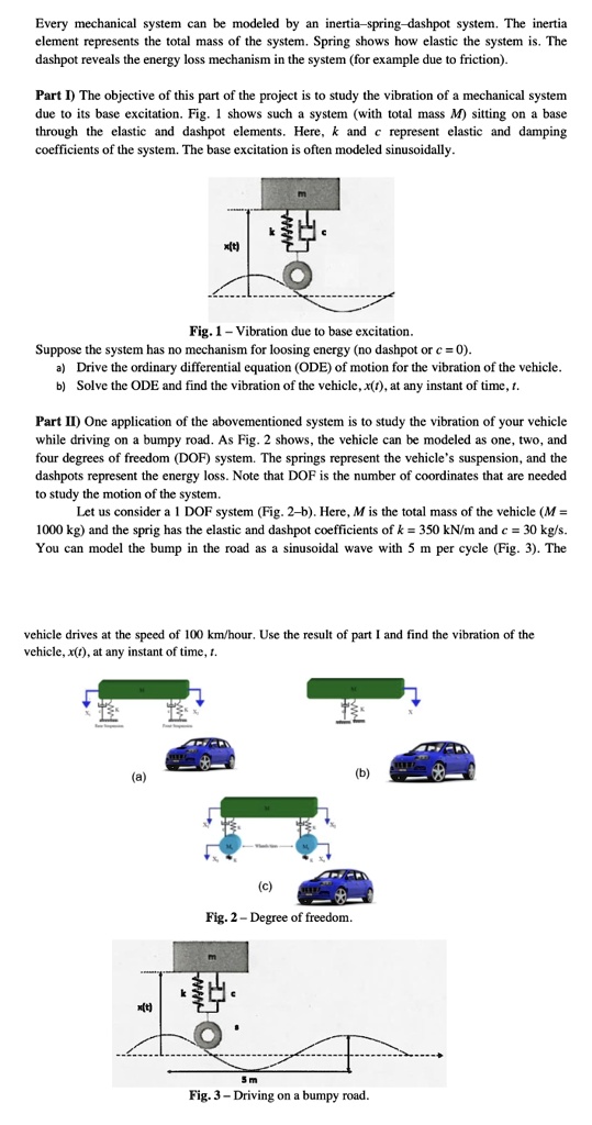
due to its base excitation. Fig. 1 shows such a system (with total mass M) sitting on a base
through the elastic and dashpot elements. Here, k and c represent elastic and damping
coefficients of the system. The base excitation is often modeled sinusoidally.
x(t)
Fig. 1-Vibration due to base excitation.
Suppose the system has no mechanism for loosing energy (no dashpot or c = 0).
a) Drive the ordinary differential equation (ODE) of motion for the vibration of the vehicle.
b) Solve the ODE and find the vibration of the vehicle, x(t), at any instant of time, t.
Part II) One application of the abovementioned system is to study the vibration of your vehicle
while driving on a bumpy road. As Fig. 2 shows, the vehicle can be modeled as one, two, and
four degrees of freedom (DOF) system. The springs represent the vehicle's suspension, and the
dashpots represent the energy loss. Note that DOF is the number of coordinates that are needed
to study the motion of the system.
Let us consider a 1 DOF system (Fig. 2-b). Here, M is the total mass of the vehicle (M =
1000 kg) and the sprig has the elastic and dashpot coefficients of k = 350 kN/m and c = 30 kg/s.
You can model the bump in the road as a sinusoidal wave with 5 m per cycle (Fig. 3). The
vehicle drives at the speed of 100 km/hour. Use the result of part I and find the vibration of the
vehicle, x(t), at any instant of time, 1.
(a)
(b)
x(t)
(c)
Fig. 2- Degree of freedom.
5 m
Fig. 3-Driving on a bumpy road.
```