University of Waterloo
Electrical and Computer Engineering
2016
E1.3C-2016: Physical Electronics
Homework 1
1D and 2D Time Function Simulation in Matlab
The objective of this homework is to solve the 1D and 2D time-dependent Schrodinger equations using Matlab to qualitatively observe the wave function corresponding to different energy states and determine the energy state specific position, energy and velocity of a particle confined in a box.
1D Problem
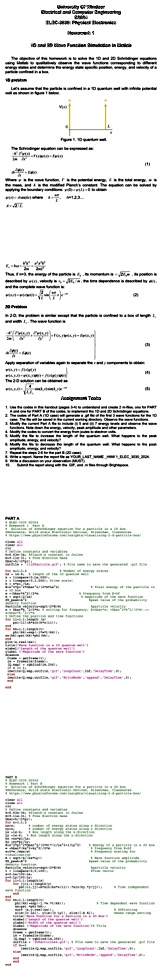
Let's assume that the particle is confined in a 1D quantum well with infinite potential well as shown in figure 1 below.
$$V(x) = \begin{cases}
0 & 0 < x < L \\
\infty & \text{otherwise}
\end{cases}$$
Figure 1. 1D quantum well
The Schrodinger equation can be expressed as
$$\frac{-\hbar^2}{2m} \frac{\partial^2}{\partial x^2} \Psi(x,t) + V(x) \Psi(x,t) = i\hbar \frac{\partial}{\partial t} \Psi(x,t)$$
(1)
Where $\Psi$ is the wave function, $V$ is the potential energy, $E$ is the total energy, $m$ is the mass, and $\hbar$ is the reduced Planck's constant. The equation can be solved by applying the boundary conditions $\Psi(0,t) = 0$ to obtain
$$\Psi(x,t) = A sin(k_nx) e^{-i\omega_nt}$$
where
$$k_n = \frac{n\pi}{L}$$
$$E_n = \frac{\hbar^2 k_n^2}{2m} = \frac{n^2 h^2}{8mL^2}$$
$$n = 1,2,3,...$$
Thus, if $n = 1$, the energy of the particle is $E_1$, its momentum is $p_1 = \hbar k_1$, its position is described by $x_1$, velocity is $v_1 = p_1/m$, the time dependence is described by $t$, and the complete wave function is
$$\Psi(x,t) = A sin(k_1x) e^{-i\omega_1t}$$
(2)
2D Problem
In 2D, the problem is similar except that the particle is confined to a box of length $L$ and width $L$. The wave function is
$$\frac{-\hbar^2}{2m} (\frac{\partial^2}{\partial x^2} + \frac{\partial^2}{\partial y^2}) \Psi(x,y,t) + V(x,y) \Psi(x,y,t) = i\hbar \frac{\partial}{\partial t} \Psi(x,y,t)$$
(3)
$$\Psi(x,y,t) = A sin(k_nx) sin(k_ny) e^{-i\omega_nt}$$
Apply separation of variables again to separate the $x$ and $y$ components to obtain
$$\Psi(x,y,t) = A sin(k_nx) sin(k_ny) e^{-i\omega_nt}$$
(4)
The 2D solution can be obtained as
$$\Psi(x,y,t) = \frac{2}{\sqrt{L}} sin(k_nx) sin(k_ny) e^{-i\omega_nt}$$
(5)
Assignment Tools
1. Use the codes in the handout pages 3-4 to understand and create 2 codes, one for the 1D and one for the 2D cases to generate a gif of the 1D and 2D wave functions for the 10 cases. The file will be a gif file including 10 directions. Observe the functions for the 10 cases.
2. The codes of Part A are the current working files. The codes were designed for the 1D simulation of current level.
3. Modify the code in Part A to include (i) a gif of energy levels and observe the 10 energy modes from the energy values, (ii) amplitude and other parameters.
4. Modify the code to increase energy, peak amplitude and width.
5. Modify the file to increase the length of the quantum well, what happens to the peak amplitude, the energy?
6. Modify the file to decrease the length of the quantum well, what happens to the peak amplitude, the energy?
7. Repeat the steps 2, 5 and 6 for part B (2D cases).
8. Write a report. Name your report as YOUR_LAST_NAME_FIRST_NAME_E1.3C_2016_HW1.docx.
9. Include discussion from the observation (MUST).
10. Submit the report along with the gif, and in files through Brightspace.
PART A
% E1.3C 2016 HW1
% Author: YOUR NAME
% Objective: Solve Schrodinger equation for a particle in a 1D box
% Description: Plot the wave function for a particle in a 1D box
% with given physical parameters and visualizing 1-D particle time-
% dependent wave function
clear all
close all
clc
% Define constants and variables in Matlab
hbar = 1.0545718e-34; % Reduced Planck's constant in Joules
m = 9.10938356e-31; % Free electron mass
L = 1e-9; % Length of the 1D quantum well
n = 10; % Number of energy states
x = linspace(0,L,1000); % Position
E = zeros(1,n); % Energy levels
k = zeros(1,n); % Wave number
omega = zeros(1,n); % Total energy of the particle in
% frequency of the wave function
psi = zeros(n,length(x)); % Amplitude of the wave function
v = zeros(1,n); % Spatial velocity of the particle
% from wave function
% Define the energy and time for frequency
for i = 1:n
k(i) = i*pi/L;
E(i) = hbar^2*k(i)^2/(2*m);
omega(i) = E(i)/hbar;
v(i) = hbar*k(i)/m;
psi(i,:) = sin(k(i)*x);
end
% Plot the wave function on a 1D quantum well
figure(1)
for i = 1:n
subplot(5,2,i)
plot(x,psi(i,:))
title(['Wave function of the n = ',num2str(i),' state'])
xlabel('Position (m)')
ylabel('Amplitude of the wave function')
end
% Time dependent wave function
figure(2)
for i = 1:n
t = linspace(0,1e-14,100); % Time in sec
psi_t = psi(i,:)*exp(-1i*omega(i)*t); % Time dependent wave function
for j = 1:length(t)
subplot(5,2,i)
plot(x,real(psi_t(j,:)))
title(['Wave function of the n = ',num2str(i),' state'])
xlabel('Position (m)')
ylabel('Amplitude of the wave function')
pause(0.01)
end
movie_map_matrix(:,:,i) = getframe;
end
imwrite(movie_map_matrix,'Wavefunction_1D.gif','WriteMode','append','DelayTime',0.1);
end
PART B
% E1.3C 2016 HW1
% Author: YOUR NAME
% Objective: Solve Schrodinger equation for a particle in a 2D box
% Description: Plot the wave function for a particle in a 2D box
% with given physical parameters and visualizing 2-D particle time-
% dependent wave function
clear all
close all
clc
% Define constants and variables in Matlab
hbar = 1.0545718e-34; % Reduced Planck's constant in Joules
m = 9.10938356e-31; % Free electron mass
L = 1e-9; % Length of the 2D quantum well
n = 10; % Number of energy states along a direction
x = linspace(0,L,1000); % Position along the x direction
y = linspace(0,L,1000); % Position along the y direction
E = zeros(n,n); % Energy levels
k = zeros(n,n); % Wave number
omega = zeros(n,n); % Frequency of a particle in a 2D box
psi = zeros(n,n,length(x),length(y)); % Wave function amplitude
v = zeros(n,n); % Spatial velocity of the particle
% from wave function
% Define the energy and time for frequency
for i = 1:n
for j = 1:n
k(i,j) = [i*pi/L,j*pi/L];
E(i,j) = hbar^2*(k(i,j).^2)/(2*m);
omega(i,j) = E(i,j)/hbar;
v(i,j) = hbar*k(i,j)/m;
psi(i,j,:,:) = sin(k(i,j)(1)*x).*sin(k(i,j)(2)*y);
end
end
% Time dependent wave function
figure(1)
for i = 1:n
for j = 1:n
t = linspace(0,1e-14,100); % Time in sec
psi_t = psi(i,j,:,:)*exp(-1i*omega(i,j)*t); % Time dependent wave function
for k = 1:length(t)
subplot(5,2,i)
surf(x,y,real(psi_t(k,:,:)))
title(['Wave function of the n = ',num2str(i),' state'])
xlabel('Position (m)')
ylabel('Position (m)')
zlabel('Amplitude of the wave function')
pause(0.01)
end
movie_map_matrix(:,:,i) = getframe;
end
end
imwrite(movie_map_matrix,'Wavefunction_2D.gif','WriteMode','append','DelayTime',0.1);
end