Numerade

Questions asked

INSTANT ANSWER

Could you answer these questions for me please? Thank you so much for your help 1. A 95% confidence interval is required for the difference between the average snack bar spending of movie goers on the weekend compared with weekday movie goers. Analyse only those who spend. a. Write out Levene’s test to establish whether the population variances can be assumed equal in this case. b. Write out the appropriate 95% confidence interval for the difference between the average snack bar spending of movie goers in the weekend compared with weekday movie goers, using the correct notation. c. Interpret the confidence interval in context. d. Show that the necessary conditions hold for the confidence interval to be valid

View Answer

INSTANT ANSWER

Descriptives Statistics Table: $ 95 \% $ Confidence Interval - Lei Frequency Table of Sessiontime - Lei Group Statistics \begin{tabular}{rl|r|r|r|r} & Weekday & $ \mathrm{N} $ & Mean & Std. Deviation & Std. Error Mean \\ \hline \multirow{2}{*}{ DAY } & Weekend & 163 & 6.21 & .408 & .032 \\ \cline { 2 - 6 } & Weekday & 173 & 3.25 & 1.519 & .115 \\ \hline \end{tabular}

View Answer

ANSWERED

Sheryl Ezze

Numerade educator

View Answer

ANSWERED

Keondre Parker

Numerade educator

Descriptives Statistics Table: 95% Confidence Interval - Lei GENDER Statistic Std. Error SNACKBAR Female Mean $6.6523 $0.16327 95% Confidence Interval for Lower Bound $6.3300 Mean Upper Bound $6.9746 5% Trimmed Mean $6.5426 Median $6.5000 Variance 4.585 Std. Deviation $2.14125 Minimum $2.50 Maximum $14.00 Range $11.50 Interquartile Range $3.00 Skewness .935 .185 Kurtosis 1.308 .368 Male Mean $7.2372 $0.22725 95% Confidence Interval for Lower Bound $6.7885 Mean Upper Bound $7.6859 5% Trimmed Mean $7.1762 Median $7.0000 Variance 8.469 Std. Deviation $2.91021 Minimum $2.00 Maximum $15.00 Range $13.00 Interquartile Range $5.00 Skewness .217 .190 Kurtosis -.721 .377 Frequency Table of Sessiontime - Lei Frequency Percent Cumulative Percent Valid Morning (before noon) 10 2.18% 2.18% Afternoon (12 noon - 5 pm inclusive) 138 30.13% 32.31% Evening (after 5 pm and before 10 pm) 264 57.64% 89.96% Late (10 pm or later) 46 10.04% 100.00% Total 458 100.00% Group Statistics Weekday N Mean Std. Deviation Std. Error Mean DAY Weekend 163 6.21 .408 .032 Weekday 173 3.25 1.519 .115

View Answer

ANSWERED

Sheryl Ezze

Numerade educator

View Answer

ANSWERED

Lucas Finney

Numerade educator

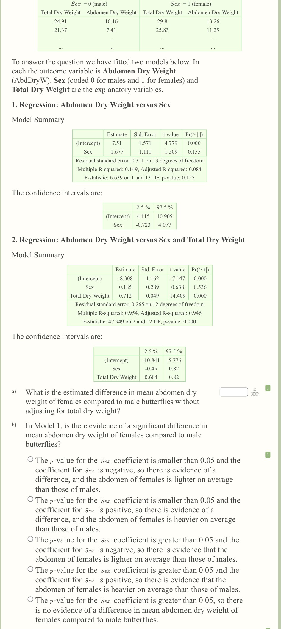
To answer the question we have fitted two models below. In each the outcome variable is Abdomen Dry Weight (AbdDryW). Sex (coded 0 for males and 1 for females) and Total Dry Weight are the explanatory variables. 1. Regression: Abdomen Dry Weight versus Sex Model Summary Estimate Std. Error t value Pr(>|t|) (Intercept) 7.51 1.571 4.779 0.000 Sex 1.677 1.111 1.509 0.155 Residual standard error: 0.311 on 13 degrees of freedom Multiple R-squared: 0.149, Adjusted R-squared: 0.084 F-statistic: 6.639 on 1 and 13 DF, p-value: 0.155 The confidence intervals are: 2.5 % 97.5 % (Intercept) 4.115 10.905 Sex -0.723 4.077 2. Regression: Abdomen Dry Weight versus Sex and Total Dry Weight Model Summary Estimate Std. Error t value Pr(>|t|) (Intercept) -8.308 1.162 -7.147 0.000 Sex 0.185 0.289 0.638 0.536 Total Dry Weight 0.712 0.049 14.409 0.000 Residual standard error: 0.265 on 12 degrees of freedom Multiple R-squared: 0.954, Adjusted R-squared: 0.946 F-statistic: 47.949 on 2 and 12 DF, p-value: 0.000 The confidence intervals are: 2.5 % 97.5 % (Intercept) -10.841 -5.776 Sex -0.45 0.82 Total Dry Weight 0.604 0.82 a) What is the estimated difference in mean abdomen dry weight of females compared to male butterflies without adjusting for total dry weight? b) In Model 1, is there evidence of a significant difference in mean abdomen dry weight of females compared to male butterflies? - The p-value for the Sex coefficient is smaller than 0.05 and the coefficient for Sex is negative, so there is evidence of a difference, and the abdomen of females is lighter on average than those of males. - The p-value for the Sex coefficient is smaller than 0.05 and the coefficient for Sex is positive, so there is evidence of a difference, and the abdomen of females is heavier on average than those of males. - The p-value for the Sex coefficient is greater than 0.05 and the coefficient for Sex is negative, so there is evidence that the abdomen of females is lighter on average than those of males. - The p-value for the Sex coefficient is greater than 0.05 and the coefficient for Sex is positive, so there is evidence that the abdomen of females is heavier on average than those of males. - The p-value for the Sex coefficient is greater than 0.05, so there is no evidence of a difference in mean abdomen dry weight of females compared to male butterflies.

View Answer

ANSWERED

Kari Hasz

Numerade educator

egin{tabular}{|c|cc|c|} hline & Lift & Stairs & Total \ hline Morning-peak & 210 & 210 & 420 \ Off-peak & 232 & 130 & 362 \ Evening-peak & 304 & 213 & 517 \ hline Total & 746 & 553 & 1299 \ hline end{tabular} The chi-squared test can be used to check to see if the choice of stairs or lift depends on the time of day. a) Select the appropriate pair of null and alternative hypotheses for this study: ( H_{0} ) : There are differences between the choice of stairs or lift and the time of day. ( H_{A} ) : There are no differences between the choice of stairs or lift and the time of day. ( H_{0} ) : Choice of stairs or lift depends on the time of day. ( H_{A} ) : Choice of stairs or lift is independent of time of day. ( H_{0} ) : Choice of stairs or lift is independent of time of day. ( H_{A} ) : Choice of stairs or lift depends on the time of day. ( H_{0} ) : There are no differences between the choice of stairs or lift and the time of day. ( H_{A} ) : There is at least one difference between the choice of stairs or lift and the time of day. ( H_{0} ) : There is an association between the choice of stairs or lift and the time of day. ( H_{A} ) : There is no association between the choice of stairs or lift and the time of day. b) Calculate the expected cell counts if the null hypothesis were true for: (i) the "Lift/Morning" cell (ii) the "Stairs/Morning" cell (iii) the "Lift/Off" cell (iv) the "Stairs/Off" cell (v) the "Lift/Evening" cell (vi) the "Stairs/Evening" cell c) Calculate the ( chi^{2} ) statistic (use your answers from b) in this calculation). d) What are the degrees of freedom for this chi-squared test? e) What line of code gives the ( p )-value for this test? 1-pchisq ( left(chi^{2}, 2 ight) ) 1 -pchisq ( left(chi^{2}, 2 ight. ), lower.tail=FALSE ( ) ) ( operatorname{pchisq}left(chi^{2}, 1 ight) ) ( operatorname{pchisq}left(chi^{2}, 1 ight. ), lower.tail=FALSE ( ) ) ( operatorname{pchisq}left(chi^{2}, 2 ight) ) f) If the significance level in our hypothesis test was 0.05 and the ( p )-value calculated from the test statistic above was less than 0.05 , select the appropriate interpretation from the options below: There is evidence at the 0.05 significance level that choice of stairs or lift depends on the time of day. There is no evidence at the 0.05 significance level that choice of stairs or lift depends on the time of day. There is evidence at the 0.05 significance level of a difference between the choice of stairs or lift and the time of day. There is evidence at the 0.05 significance level of at least one difference between the choice of stairs or lift and the time of day. There is insufficient evidence at the 0.05 significance level of a difference between the choice of stairs or lift and the time of day.

View Answer

ANSWERED

Qudsiya Anis

Numerade educator

A team of eye surgeons have developed a new technique to restore the sight of people blinded from a certain disease. Under the old method it is known that only 31% of patients who undergo this operation recover their eyesight. In a random sample of 299 operations performed using the new method, 100 patients fully recovered their eyesight. a) Select the appropriate null and alternative hypotheses for investigating whether the new method is any different to the old one. π denotes the population proportion that improve under the new method, and p denotes the proportion that improved under the new method within the sample above. 1) H0 : π ≠ 0.31 ; HA : π = 0.31 2) H0 : π = 0.31 ; HA : π ≠ 0.31 3) H0 : μ = 0.31 ; HA : μ ≠ 0.33 4) H0 : p = 0.31 ; HA : p ≠ 0.31 5) H0 : π = 0.33 ; HA : π ≠ 0.33 b) What proportion of patients had their eyesight recovered in the new method in the sample. c) Find the standardized test statistic for this study. d) Calculate the p-value for this test. e) Given the p-value calculated in part d) and α=0.05, select the conclusion which would be appropriate for this hypothesis test. 1) The p-value is greater than or equal to 0.05. There is evidence to reject H0. There is evidence to suggest the percentage who recover their eyesight with the new method is different to the percentage who recover their eyesight under the old method. 2) The p-value is less than 0.05. There is evidence to reject H0. There is evidence that the percentage who recover their eyesight with the new method is different from the percentage who recover their eyesight with the old method. 3) The p-value is less than 0.05. There is insufficient evidence to reject H0. There is not sufficient evidence to conclude that the percentage who recover their eyesight with the new method is significantly different to the percentage who recover their eyesight under the old method. 4) The p-value is greater than or equal to 0.05. There is insufficient evidence to reject H0. There is not sufficient evidence to conclude that the percentage who recover their eyesight with the new method is different to the percentage who recover their eyesight under the old method.

View Answer

ANSWERED

Qudsiya Anis

Numerade educator

a) Select the appropriate null and alternative hypotheses for investigating whether the new method is any different to the old one. ? denotes the population proportion that improve under the new method, and p denotes the proportion that improved under the new method within the sample above. H0 : ? ? 0.31; HA : ? = 0.31 H0 : ? = 0.31; HA : ? ? 0.31 H0 : ? = 0.31; HA : ? ? 0.33 H0 : p = 0.31; HA : p ? 0.31 H0 : ? = 0.33; HA : ? ? 0.33 b) What proportion of patients had their eyesight recovered in the new method in the sample. c) Find the standardized test statistic for this study. d) Calculate the p-value for this test. e) Given the p-value calculated in part d) and ? = 0.05, select the conclusion which would be appropriate for this hypothesis test. The p-value is greater than or equal to 0.05. There is evidence to reject H0. There is evidence to suggest the percentage who recover their eyesight with the new method is different to the percentage who recover their eyesight under the old method. The p-value is less than 0.05. There is evidence to reject H0. There is evidence that the percentage who recover their eyesight with the new method is different from the percentage who recover their eyesight with the old method. The p-value is less than 0.05. There is insufficient evidence to reject H0. There is not sufficient evidence to conclude that the percentage who recover their eyesight with the new method is significantly different to the percentage who recover their eyesight under the old method. The p-value is greater than or equal to 0.05. There is insufficient evidence to reject H0. There is not sufficient evidence to conclude that the percentage who recover their eyesight with the new method is different to the percentage who recover their eyesight under the old method.

View Answer

ANSWERED

Robin Corrigan

Numerade educator

In a study, 45 smokers were questioned about the number of hours they sleep each day. For the sample of smokers, the mean number of hours slept per day was 7.4 hours and the standard deviation was 1 hours. We wish to test the hypothesis that smokers have a different amount of sleep than the general public, who sleep for an average of 7.5 hours per day. Use ( alpha=0.05 ). a) Which one of the following is the appropriate pair of hypotheses? [ egin{array}{ll} H_{0}: mu=7.5 ; & H_{A}: mu eq 7.5 \ H_{0}: mu=7.4 ; & H_{A}: mu=7.5 \ H_{0}: mu=7.4 ; & H_{A}: mu eq 7.4 \ H_{0}: ar{x}=7.5 ; & H_{A}: ar{x} eq 7.5 \ H_{0}: ar{x}=7.4 ; & H_{A}: ar{x} eq 7.4 end{array} ] b) Calculate the standardized test statistic for this study. ( 3 mathrm{DP} ) c) Find the ( p )-value associated with the test statistic. d) From the ( p )-value you found above, select the appropriate conclusion for an hypothesis test carried out at the ( alpha=5 % ) significance level: As the ( p )-value is greater than or equal to 0.05 , there is no evidence at the 0.05 -significance level to reject ( H_{0} ) : i.e. there is no evidence that smokers sleep more or less than the general population. The observed difference is within the range we would expect due to random variation. As the ( p )-value is less than 0.05 , there is no evidence at the 0.05 -significance level to reject ( H_{0} ). The observed difference is within the range we would expect due to random variation. As the ( p )-value is less than 0.05 , we have evidence at the 0.05 -significance level that the true amount of sleep in the general population is more than 7.5 hours per night. As the ( p )-value is less than 0.05 , there is evidence to reject ( H_{0} ) at the 0.05 -significance level, which suggests that the true mean hours of sleep for smokers is different from the general population. We have evidence that ( 7.4 % ) of smokers sleep more than the general public.

View Answer

Sina L.