Use the following to answer questions 25-26:
\table[[\table[[Expected rate],[of return (%)]],\table[[RUse the following to answer questions 25-26:
\table[[\table[[Expected rate],[of return (%)]],\RUse the following to answer questions 25-26:
\table[[\table[[Expected rate],[of return (%)]],\table[[RUse the following to answer questions 25-26:
\table[[\table[[Expected rate],[of return (%)]],\table[[R
Use the following to answer questions 25-26:
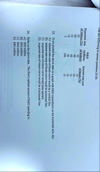
\table[[\table[[Expected rate],[of return (%)]],\table[[R&D],[(millions],[of dollars)]],\table[[Interest rate cost],[of funds (%)]],],[25,,20,10],[20,,40,10],[15,,60,10],[10,,80,10],[5,,100,10]]
If we plotted the above data on a graph with R&D expenditures on the horizontal axis, the:
A) interest-rate-cost-of-funds-curve would be a vertical line.
B) interest-rate-cost-of-funds-curve would be horizontal line.
C) expected-rate-of-return-curve would slope upward.
D) expected-rate-of-return-curve would be a horizontal line.
Refer to the above data. The firm's optimal amount of R&D spending is:
A) $20 million.
B) $40 million.
C) $60 million.
D) $80 million.