Here I also want to know the step-by-step that you used to find the transfer function and why are the parameters of the transfer function very large? Also, help me to find the transfer function that enables me to design the controller for this linearized system.
Explanation:
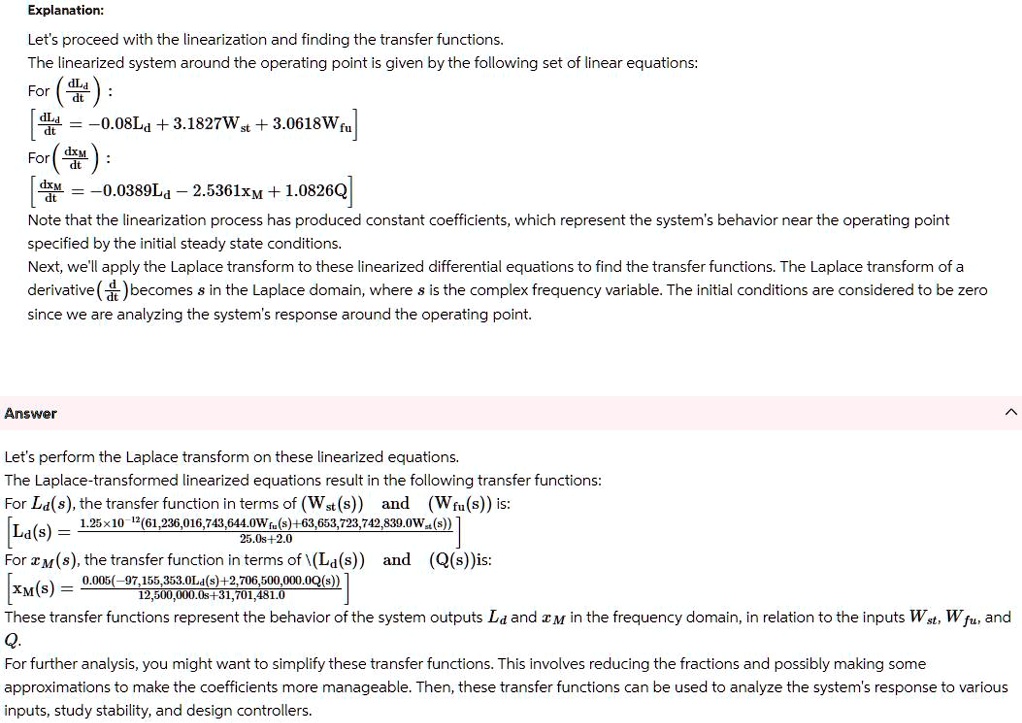
Let's proceed with the linearization and finding the transfer functions. The linearized system around the operating point is given by the following set of linear equations:
-0.08La + 3.1827Wst + 3.0618Wfu = -0.0389L - 2.5361xM + 1.0826Q.
Note that the linearization process has produced constant coefficients, which represent the system's behavior near the operating point specified by the initial steady state conditions. Next, we'll apply the Laplace transform to these linearized differential equations to find the transfer functions. The Laplace transform of a derivative (d/dt) becomes s in the Laplace domain, where s is the complex frequency variable. The initial conditions are considered to be zero since we are analyzing the system's response around the operating point.
Answer:
Let's perform the Laplace transform on these linearized equations. The Laplace-transformed linearized equations result in the following transfer functions: For Las, the transfer function in terms of Wst and Wfu is:
25.0s^2.
For Ms, the transfer function in terms of Las and Q is:
12,500,000.0s + 31,701,481.
These transfer functions represent the behavior of the system outputs Ia and in the frequency domain, in relation to the inputs Wst, Wfu, and Q. For further analysis, you might want to simplify these transfer functions. This involves reducing the fractions and possibly making some approximations to make the coefficients more manageable. Then, these transfer functions can be used to analyze the system's response to various inputs, study stability, and design controllers.